III Halo 2 Guide: The Halo 2 proof system, from arithmetisation to recursion 6 The verifier’s decision and its implication chain IV Consensus Guide: Nakamoto consensus: the double-spend race, the arithmetic of confirmations, and the deployed most-work rule

7 Recursive proof composition and accumulation schemes

This section states recursive proof composition and accumulation for the inner-product argument; Orchard deploys neither. The protocol specification uses Halo 2 for one purpose, to prove and verify Action statements (protocol specification, § 4.1.13, “Zero-Knowledge Proving System”), and requires every Action proof to be valid (§ 4.6, “Action Descriptions”); the design proposal that introduced the pool states that it makes no use of the proof system’s support for recursive proofs (ZIP 224, under “Proving system”). A verifier holding several proofs may still check them together. The complete verification equation $E_{i}$ of each proof is a multi-scalar multiplication over all $d$ generators that should evaluate to $\mathcal{O}$ (§3.8.1, “Batch verification”); for independent uniform $\mu_{1},\dots,\mu_{b}\in\mathbb{F}$ the verifier of $b$ proofs checks $\sum_{i}[\mu_{i}]\,E_{i}=\mathcal{O}$ instead. If some $E_{j}\neq\mathcal{O}$ , then $E_{j}$ generates the group of prime order, so for any fixed values of the other factors exactly one $\mu_{j}$ satisfies the combined check, and a false batch passes with probability $1/|\mathbb{F}|$ (Lemma 3.14). Batch verification verifies the batch and emits nothing; it is not the accumulation developed here. In the classification of §1.2, the Pasta curves and the use Orchard makes of them (§7.4) are specified; recursion and accumulation over those curves are designed-but-unspecified: their constructions are published and the halo2 book describes them (Recursion chapter), and ZIP 224 leaves them to future protocol updates, but no specification defines a recursive statement or an accumulation rule for Zcash. Theorem 7.4 and Proposition 7.5 below are theorems, the first cited and the second proved.

7.1 Recursion and its two classical obstacles

The setting.

Consider a computation iterated many times,

z_{m}=f^{(m)}(z_{0}):=f\bigl{(}f(\cdots f(z_{0})\cdots)\bigr{)},

one step $f$ applied $m$ times to an initial state, and suppose a verifier wants to be sure that $z_{m}$ is the honest result without recomputing the $m$ steps. Valiant’s incrementally verifiable computation asks for a proof of $z_{m}$ that is updated step by step, each update costing about one step’s worth of proving and the finished proof no larger than the proof of a single step. The more general setting, in which computations branch and merge and each step consumes the proofs of its predecessors, is the proof-carrying data of Chiesa and Tromer: every message in a distributed computation carries a proof that it was produced correctly from messages that themselves carried such proofs.

The construction.

The natural construction is recursive proof composition: proving, inside one proof, that another proof verifies. Write $\mathcal{V}$ for the verifier of a non-interactive argument (Crypto Guide, §“SNARKs: succinct non-interactive arguments of knowledge”), and suppose its algorithm is itself arithmetised, in the sense of §2, into a PLONKish circuit of Definition 2.7, the verifier circuit: its instance columns hold the statement and its advice columns hold a proof, and its gates are satisfiable exactly when $\mathcal{V}$ accepts that proof of that statement. At step $i+1$ the prover proves the compound statement

“ $z_{i+1}=f(z_{i})$ , and there exists a proof $\pi_{i}$ that the verifier circuit accepts for the statement of step $i$ .”

The proof $\pi_{i}$ is advice of the step- $(i+1)$ circuit, never sent onward; the proof $\pi_{i+1}$ that results attests to step $i+1$ and, through the embedded verifier, to $\pi_{i}$ , hence to step $i$ , and so on down to $z_{0}$ . One proof attests to the entire history, and the cost of producing $\pi_{i+1}$ is the cost of one step of $f$ plus one run of the verifier circuit, independent of how long the history is. The requirement on which everything rests is the one just used: the argument’s verifier must be efficiently expressible as a circuit. A verifier whose circuit is as large as the computation it checks would make each step as expensive as the whole history, and the construction would buy nothing.

Two obstacles.

The classical instantiations meet that requirement badly, in two different ways.

1.

Pairings in a circuit, and a ceremony. The pairing-based systems, Groth16, which Sapling deploys, and PLONK compiled with the KZG commitment (Crypto Guide, §“SNARKs: succinct non-interactive arguments of knowledge” for Groth16 and the bilinear pairing; §“Polynomial commitment schemes”, under “KZG: evaluation in the exponent”), have constant-size proofs and verifiers that run in time independent of the circuit. But those verifiers evaluate pairings, and a pairing lands in a target group that lives in an extension field $\mathbb{F}_{p^{e}}$ of the curve’s base field, of degree $e$ equal to the curve’s embedding degree (Crypto Guide, §“Instantiation on elliptic curves; the Pasta curves”, the large-embedding-degree criterion). A circuit whose native arithmetic is one prime field must emulate arithmetic in another field with many gates per operation, so a pairing is costly to express inside a circuit. These particular systems also need a trusted setup, the ceremony that §3.8.1 contrasted with hashed generators.
2.

A linear-time verifier. The transparent systems built on the inner-product argument of §3 need no pairing and no ceremony, but their verifier is linear in the size of the committed vectors: the one multi-scalar multiplication $G^{(0)}=\langle\mathbf{s},\,\mathbf{G}\rangle$ of length $d$ that §3.4 singled out. Inside a verifier circuit that multiplication is $d$ scalar multiplications of curve points, each a double-and-add with $\ell-1$ doublings for an $\ell$ -bit scalar (Math Guide, §“Scalar multiplication and double-and-add”), so the verifier circuit grows linearly in $d$ , the length of the committed vectors of the proof it verifies. A linear-time check dominates the verifier circuit and negates the per-step economy that recursion was meant to deliver.

Deferred verification.

Halo, the construction of Bowe, Grigg and Hopwood (Halo: Recursive Proof Composition without a Trusted Setup) from which Halo 2 descends, defers the linear-time part of verification instead of recomputing it at every step, and uses the inner-product argument, in which no pairing occurs. Bünz, Chiesa, Mishra and Spooner formalised the deferral as an accumulation scheme (Proof-Carrying Data from Accumulation Schemes; BCMS20), the notion the next subsection defines; their Theorem 7.1 is quoted below, without proof, as Theorem 7.4.

7.2 Accumulation schemes

The idea is to separate what a verifier must check at each step from what can be checked once, at the end of a chain. Fix a predicate $\Phi$ , a property of an input $q$ decidable in polynomial time, for example “this inner-product opening is correct” of a transcript of Construction 3.2. An accumulation scheme replaces a sequence of checks of $\Phi$ by a sequence of accumulation steps and one run of a decider.

Definition 7.1 (Accumulation scheme).

Let $\lambda$ be the security parameter (Crypto Guide, §“Adversaries and the security parameter”) and $\Phi$ a predicate on inputs $q$ . An accumulation scheme for $\Phi$ is a triple $(\mathsf{P},\mathsf{V},\mathsf{D})$ of polynomial-time algorithms with access to a common random oracle, whose accumulators are bit strings.

1.

The accumulation prover $\mathsf{P}$ , on input $q$ and an old accumulator $\mathsf{acc}_{\mathrm{old}}$ , outputs a new accumulator $\mathsf{acc}$ and an accumulation proof $\pi_{\mathsf{V}}$ .
2.

The accumulation verifier $\mathsf{V}$ , on input $(q,\mathsf{acc}_{\mathrm{old}},\mathsf{acc},\pi_{\mathsf{V}})$ , outputs a bit; the bit $1$ asserts that $\mathsf{acc}$ correctly accumulates $q$ and $\mathsf{acc}_{\mathrm{old}}$ .
3.

The decider $\mathsf{D}$ , on input an accumulator, outputs a bit; an accumulator is valid if $\mathsf{D}$ outputs $1$ on it.

The scheme is complete if, whenever $\Phi(q)=1$ , $\mathsf{D}(\mathsf{acc}_{\mathrm{old}})=1$ and $(\mathsf{acc},\pi_{\mathsf{V}})$ is an output of $\mathsf{P}$ on $(q,\mathsf{acc}_{\mathrm{old}})$ , both $\mathsf{V}(q,\mathsf{acc}_{\mathrm{old}},\mathsf{acc},\pi_{\mathsf{V}})=1$ and $\mathsf{D}(\mathsf{acc})=1$ . It is sound if for every adversary of size polynomial in $\lambda$ that outputs $(q,\mathsf{acc}_{\mathrm{old}},\mathsf{acc},\pi_{\mathsf{V}})$ the probability, over the random oracle and the adversary’s coins, of

\mathsf{V}(q,\mathsf{acc}_{\mathrm{old}},\mathsf{acc},\pi_{\mathsf{V}})=1\;% \wedge\;\mathsf{D}(\mathsf{acc})=1\;\wedge\;\bigl{(}\Phi(q)=0\,\vee\,\mathsf{D% }(\mathsf{acc}_{\mathrm{old}})=0\bigr{)}

is negligible in $\lambda$ .

The definition is that of BCMS20 (Section 4.1) with one input and one old accumulator per step; theirs admits any number of each and adds a generator and an indexer, which fix the public parameters and keys left implicit here. For recursion the size of an accumulator must also be bounded independently of the number of inputs accumulated into it (BCMS20, Definition 5.1).

Soundness carries the checks along a chain.

Lemma 7.2 (Soundness along a chain).

Let $(\mathsf{P},\mathsf{V},\mathsf{D})$ be sound in the sense of Definition 7.1, let $\mathsf{acc}_{0}$ be valid, and let $m$ be polynomial in $\lambda$ . For any efficient algorithm producing $q_{1},\dots,q_{m}$ and $\mathsf{acc}_{1},\dots,\mathsf{acc}_{m}$ , where $\mathsf{acc}_{i}$ accumulates $q_{i}$ and $\mathsf{acc}_{i-1}$ , such that $\mathsf{V}$ accepts every step and $\mathsf{D}(\mathsf{acc}_{m})=1$ , the probability that $\Phi(q_{i})=0$ for some $i$ is at most $m$ times the soundness error of the adversary that outputs step $i$ for a uniform $i\in\{1,\dots,m\}$ ; it is therefore negligible.

Proof.

If some $q_{i}$ violates $\Phi$ , then either $\mathsf{acc}_{i}$ is valid and step $i$ exhibits the event of the soundness definition, or some later step $j>i$ turns an invalid $\mathsf{acc}_{j-1}$ into a valid $\mathsf{acc}_{j}$ and exhibits it. Let $\mathcal{A}$ be the algorithm that produces the chain and outputs step $i$ for a uniform $i\in\{1,\dots,m\}$ ; since the bad event forces some step to exhibit the soundness event, its probability is at most $m$ times the soundness error of $\mathcal{A}$ , which is negligible because $m$ is polynomial (Math Guide, §“Polynomial, exponential, and negligible functions”, the closure properties). □

The verifier of each step runs the accumulation verifier and never the decider. In a recursive chain the accumulation verifier runs inside the circuit of the step’s proof, so the argument also needs the knowledge soundness of each step’s proof, to recover what that circuit checked; BCMS20 prove the resulting proof-carrying data secure for computations of constant depth, which for a chain means constant length, because the extractor is applied recursively once per level (Theorem 5.2 and Remark 5.3).

For an inner-product polynomial commitment such a scheme is known under the hypothesis of Theorem 7.4 below, and it resolves the second obstacle of §7.1 where it arose: the verifier circuit runs the $O(\log d)$ part of the opening check, the rounds, the scalars and the small combinations of points, and accumulates the $O(d)$ part, the claim about $G^{(0)}$ , into a running accumulator; the decider pays that multi-scalar multiplication once, at the end of the chain. The next subsection defines the accumulator, states the scheme as an interface theorem, and works the fold on the toy curve.

7.3 Accumulation and the Halo trick

The asymmetry, recalled.

Everything the verifier of Construction 3.2 does to decide the check (15), or its deployed form (29), is logarithmic in $d$ : $3k-2$ field multiplications for $g(x;\mathbf{u})$ , a combination of the $2k$ received points and a handful of fixed ones with $O(k)$ scalar multiplications, and a comparison of two curve points. The single exception is the evaluation

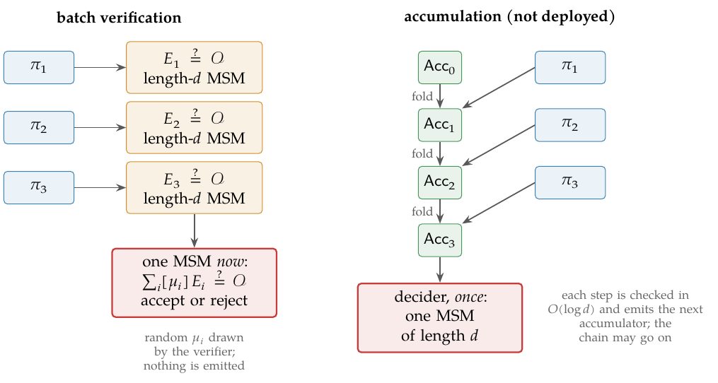
G^{(0)}=\langle\mathbf{s},\,\mathbf{G}\rangle=\mathsf{Commit}\bigl{(}g(X;\,u_{% 1},\dots,u_{k});\,0\bigr{)},

a multi-scalar multiplication of length $d$ over all the generators, which §3.4 named the one linear step and recognised as the unblinded commitment to the polynomial $g$ whose value the verifier had just computed cheaply. Verifying an Action proof as the consensus rules require includes that step for every proof; batch verification, recalled at the start of this section, evaluates one combined multiplication for the proofs of a batch, and the batch is verified and nothing survives it. Accumulation takes the same kind of linear combination and does something else with it: it carries the combined claim forward as data, unverified, and pays for it once at the end of a chain. Figure 18 sets the two side by side; the rest of this subsection is the right-hand panel, and none of it is deployed by Orchard.

Refer to caption — Figure 18: Left: batch verification. Each proof’s complete verification equation $E_{i}$ is a multi-scalar multiplication over the $d$ generators (amber); the verifier combines them with fresh random factors and evaluates one multiplication immediately (red), then accepts or rejects. Right: accumulation. Each proof’s deferred claim is accumulated into a running accumulator (green), each step being checked at logarithmic cost; the accumulator is emitted for the next step, and a decider evaluates one length- $d$ multiplication at the end of the chain. Both take random linear combinations; only the right-hand scheme carries a claim forward.

The atomic accumulator.

The claim to be deferred has a fixed shape, and the accumulator is that shape written down.

Definition 7.3 (Atomic accumulator for the inner-product argument).

An accumulator instance is a tuple

\mathsf{Acc}:=\bigl{(}G^{(0)},u_{1},\dots,u_{k}\bigr{)}\in\mathbb{G}\times(% \mathbb{F}^{\times})^{k},

a curve point and the $k$ round challenges of one opening. It is valid if and only if

G^{(0)}=\langle\mathbf{s}(\mathbf{u}),\,\mathbf{G}\rangle=\mathsf{Commit}\bigl% {(}g(X;\,u_{1},\dots,u_{k});\,0\bigr{)},

(35)

with $\mathbf{s}(\mathbf{u})$ and $g$ the structured scalars and the polynomial of Theorem 3.3, in the symmetric normalisation of Construction 3.2. The deferred claim concerns the unblinded commitment: the blinder of the opened commitment was discharged by the $[r^{*}]H$ term of (15), or the $[f]H$ term of (29), and plays no part in it. From here on the unary $\mathsf{Commit}(\cdot)$ abbreviates $\mathsf{Commit}(\cdot\,;\,0)$ .

The deployed analogue replaces $\mathbf{s}(\mathbf{u})$ and $g$ by their forms in Remark 3.9; Proposition 7.5 and, with verifier-drawn challenges, the closure argument below hold for it verbatim, with Corollary 3.13 in place of Theorem 3.5, since they use only the linearity of the commitment, the degree of $g$ and the knowledge soundness of the opening.

A verifier who is handed a point $G^{(0)}$ together with the challenges can complete the check (15) in $O(\log d)$ operations provided the tuple is valid; validity is precisely what he has not paid for. The scheme quoted next lets him defer that payment.

Theorem 7.4 (Accumulation for the inner-product argument; interface).

Let $\mathrm{PC}_{\mathrm{DL}}$ be the inner-product polynomial commitment of BCMS20 (Appendix A.2), for polynomials of degree below $d$ over a group $\mathbb{G}$ of prime order, and suppose that $\mathrm{PC}_{\mathrm{DL}}$ is a polynomial commitment scheme in the random oracle model, its openings in particular being extractable. Then (BCMS20, Theorem 7.1) there is an accumulation scheme in the sense of Definition 7.1, in the random oracle model, for the predicate “this $\mathrm{PC}_{\mathrm{DL}}$ opening is correct”, whose accumulators are themselves $\mathrm{PC}_{\mathrm{DL}}$ openings, such that:

1.

the accumulation prover $\mathsf{P}$ runs in time dominated by $O(d)$ scalar multiplications in $\mathbb{G}$ ;
2.

the accumulation verifier $\mathsf{V}$ runs in time dominated by $O(\log d)$ scalar multiplications in $\mathbb{G}$ ;
3.

the decider $\mathsf{D}$ is the opening check of $\mathrm{PC}_{\mathrm{DL}}$ : a succinct part, which yields a tuple of the form of Definition 7.3 in the normalisation of Remark 3.9, followed by the validity check (35) of that tuple, one multi-scalar multiplication of length $d$ .

The theorem is quoted as an interface and not proved in this volume. Its hypothesis, the extractability of $\mathrm{PC}_{\mathrm{DL}}$ openings, is stated by BCMS20 as a conjecture from the binding of the Pedersen commitment, the extractor they record for the Fiat–Shamir-compiled opening running in superpolynomial time (BCMS20, Appendix A.3.2). The scheme $\mathrm{PC}_{\mathrm{DL}}$ is neither Construction 3.2, whose fold is symmetric, nor the deployed opening of Remark 3.9, which blinds every commitment and subtracts $[v]\,G_{0}$ where $\mathrm{PC}_{\mathrm{DL}}$ adds a multiple of its inner-product generator (the halo2 book’s Comparison to other work chapter); no theorem transferring it to either is proved here or cited, and in the classification of §1.2 that transfer, like accumulation over these curves, is designed-but-unspecified. What an accumulation step does for Construction 3.2, and why its random combination is sound, is worked out below at the level the volume proves things.

The accumulation step in the verifier circuit.

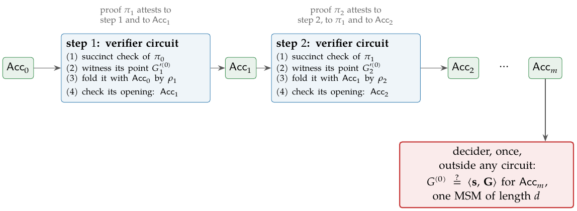
Consider a Halo 2 verifier circuit, expressed over the scalar field of one Pasta curve and verifying a proof produced over the other curve, an arrangement whose necessity §7.4 explains. At step $i$ of a chain the circuit receives the previous proof $\pi_{i-1}$ , whose opening is an instance of Construction 3.2, and the accumulator $\mathsf{Acc}_{i-1}$ exposed as a public input of $\pi_{i-1}$ , of which it uses the instance on the curve $\pi_{i-1}$ is committed on (see below), and does three things.

1.

Run the succinct part. It recomputes the challenges $\mathbf{u}^{\prime}$ of the opening from the transcript, evaluates $g(x;\mathbf{u}^{\prime})$ with $O(k)$ scalar operations, and forms the left-hand side of (15) and every term of the right-hand side except the one on the final generator, here written $G^{\prime(0)}$ , with $O(k)$ point operations. The point operations are native, since the points of $\pi_{i-1}$ have coordinates in the circuit’s field. The challenges, $g(x;\mathbf{u}^{\prime})$ and the scalar products lie in the scalar field of the curve $\pi_{i-1}$ is committed on, the other Pasta field; they are computed non-natively, or exposed as public inputs and checked by the next circuit of the chain, which is native to that field (“What the cycle does and does not buy” in §7.4; the halo2 book’s Recursion chapter).
2.

Witness the expensive part. It does not compute $G^{\prime(0)}$ . The prover of the step supplies the claimed point as advice, and the circuit uses it to complete the check, which is then passed conditionally on the validity of the fresh tuple $(G^{\prime(0)},\mathbf{u}^{\prime})$ of that opening.
3.

Accumulate. The step now holds two claims of the shape (35): the inherited instance $(G^{(0)},\mathbf{u})$ of $\mathsf{Acc}_{i-1}$ and the fresh $(G^{\prime(0)},\mathbf{u}^{\prime})$ . For a challenge $\rho$ derived by the random oracle from both tuples, the two reduce to the single claim

$G^{(0)}+[\rho]\,G^{\prime(0)}\;=\;\mathsf{Commit}\bigl{(}g(X;\mathbf{u})+\rho% \,g(X;\mathbf{u}^{\prime})\bigr{)}=\langle\mathbf{s}(\mathbf{u})+\rho\,\mathbf% {s}(\mathbf{u}^{\prime}),\,\mathbf{G}\rangle,$ (36)

whose coefficient vector on the right anyone holding both challenge tuples can recompute. Proposition 7.5 shows that a false input survives the combination for at most one $\rho$ . The step’s prover then opens the combined point at a fresh point, outside the circuit, and the circuit checks that opening succinctly as in item 1; the tuple the opening leaves behind is the new accumulator $\mathsf{Acc}_{i}$ (over a 2-cycle, its instance on that curve), exposed as a public input of the proof $\pi_{i}$ the step produces. The paragraph “Closure: the prover-assisted step” below describes that opening.

Over a 2-cycle of curves (§7.4) the proofs alternate between the two curves, and the accumulator is a pair of instances, one per curve. The step that verifies a proof committed on one curve folds that proof’s fresh tuple into the instance on the same curve, which was last updated two steps earlier and forwarded unchanged by the intervening step, and it forwards the other curve’s instance in the same way, without point arithmetic. Figure 19 draws the chain. At its end a single multi-scalar multiplication of length $d$ , run outside any circuit, checks the last accumulator and with it every opening in the history: for the scheme of Theorem 7.4 by Lemma 7.2.

Why the fold is sound.

The soundness of the fold (36) is one line of linear algebra in the group.

Proposition 7.5 (Soundness of the $\rho$ -fold).

Let $(G^{(0)},\mathbf{u})$ and $(G^{\prime(0)},\mathbf{u}^{\prime})$ be two accumulator instances and $\rho$ uniform in $\mathbb{F}$ , drawn after both are fixed. If both instances are valid, the folded equation (36) holds for every $\rho$ . If at least one is invalid, it holds for at most one value of $\rho$ , hence with probability at most $1/|\mathbb{F}|$ .

Proof.

Set $\Delta:=G^{(0)}-\mathsf{Commit}(g(X;\mathbf{u}))$ and $\Delta^{\prime}:=G^{\prime(0)}-\mathsf{Commit}(g(X;\mathbf{u}^{\prime}))$ , the two errors. By linearity of the commitment (Crypto Guide, §“Pedersen vector commitments”, the remark that linearity survives), $\mathsf{Commit}(g+\rho g^{\prime})=\mathsf{Commit}(g)+[\rho]\mathsf{Commit}(g^% {\prime})$ , so the left-hand side of (36) minus the right is $\Delta+[\rho]\,\Delta^{\prime}$ , and the equation holds exactly when

\Delta+[\rho]\,\Delta^{\prime}=\mathcal{O}.

(37)

If both instances are valid, $\Delta=\Delta^{\prime}=\mathcal{O}$ and the equation holds for all $\rho$ . Otherwise two cases. If $\Delta^{\prime}\neq\mathcal{O}$ , then, $\mathbb{G}$ being cyclic of prime order, $\Delta^{\prime}$ generates $\mathbb{G}$ and the map $\rho\mapsto[\rho]\Delta^{\prime}$ is a bijection $\mathbb{F}\to\mathbb{G}$ (Math Guide, §“The mixed inner product with group elements”, the one-dimensional vector space $\mathbb{G}$ over $\mathbb{F}$ ), so exactly one $\rho$ sends $\Delta^{\prime}$ to $-\Delta$ : the discrete logarithm of $-\Delta$ to the base $\Delta^{\prime}$ , which exists whether or not anyone can compute it. If $\Delta^{\prime}=\mathcal{O}$ , then $\Delta\neq\mathcal{O}$ and (37) holds for no $\rho$ . A uniform $\rho$ hits the at most one bad value with probability at most $1/|\mathbb{F}|$ . □

Example 7.6 (The fold on the toy curve).

The fold is run on the $97$ -point curve and the four generators $G_{0},\dots,G_{3}$ of §3.7, with $d=4$ and the symmetric structured scalars of Theorem 3.3, on two challenge tuples, $(u_{1},u_{2})=(52,44)$ with $\mathbf{s}=(80,10,68,57)$ and $G^{(0)}=\langle\mathbf{s},\,\mathbf{G}\rangle=(21,10)$ , and $(u_{1}^{\prime},u_{2}^{\prime})=(41,39)$ with $\mathbf{s}^{\prime}=(64,11,53,47)$ and $G^{\prime(0)}=(23,2)$ , both valid by construction, for every $\rho\in\mathbb{F}_{97}$ . With both instances valid the folded equation (36) holds for all $97$ values of $\rho$ . Spoiling an instance by adding a nonzero multiple of $G_{0}$ to its point makes its error $\Delta$ a nonzero point, and the surviving values of $\rho$ are counted again. With the first instance false and the second valid, no $\rho$ survives: this is the case $\Delta^{\prime}=\mathcal{O}\neq\Delta$ of the proof. With the second false and the first valid, exactly one survives, $\rho=0$ , the value that discards the second instance altogether. With both false exactly one survives, $\rho=50$ , the discrete logarithm of $-\Delta$ to the base $\Delta^{\prime}$ on this curve, where such logarithms are a short search. In every spoiled case the count is at most one of $97$ : the bound $1/|\mathbb{F}|$ of Proposition 7.5, attained.

Closure: the prover-assisted step.

The folded claim (36) is not an accumulator instance. Its coefficient vector $\mathbf{s}(\mathbf{u})+\rho\,\mathbf{s}(\mathbf{u}^{\prime})$ is in general not the structured vector of any single challenge tuple, so carrying it means carrying both tuples, and after $m$ folds all $m$ of them: the decider would still pay one multiplication of length $d$ , but the accumulator would grow with the chain, against the size bound that recursion requires (§7.2). The tuple type of Definition 7.3 is therefore not closed under verifier-side linear combination alone. It is closed under one more step, which the prover assists. Write $A:=G^{(0)}+[\rho]\,G^{\prime(0)}$ for the combined point and $a(X):=g(X;\mathbf{u})+\rho\,g(X;\mathbf{u}^{\prime})$ for the combined polynomial, of degree below $d$ . The combined claim says exactly that $A=\mathsf{Commit}(a)$ . The step’s prover opens $A$ by the opening protocol of Construction 3.2 at a fresh point $x^{\prime}$ , derived by the random oracle from $A$ and both tuples, claiming the value $a(x^{\prime})$ , which the verifier computes for himself in $O(k)$ field operations from the two tuples, since $g(x^{\prime};\mathbf{u})$ and $g(x^{\prime};\mathbf{u}^{\prime})$ are each a product of $k$ factors. That opening does two things at once. First, it carries the combined claim up to a blinder.

Proposition 7.7 (Prover-assisted step, verifier-drawn challenges).

Under the hypotheses of Theorem 3.5, let $\rho$ , $x^{\prime}$ and the opening’s challenges be drawn uniformly by the verifier, in this order, $\rho$ after the two tuples are fixed. There is an extractor which, given rewindable access to a step prover accepted with non-negligible probability, runs in expected polynomial time and outputs either blinders $\delta,\delta^{\prime}$ with $G^{(0)}=\mathsf{Commit}(g(X;\mathbf{u});\,\delta)$ and $G^{\prime(0)}=\mathsf{Commit}(g(X;\mathbf{u}^{\prime});\,\delta^{\prime})$ , or a nontrivial discrete-logarithm relation among $\mathbf{G}$ , $H$ , $U$ , $U^{\prime}$ . Its knowledge error is $O(\log d/|\mathbb{F}|)+(d-1)/|\mathbb{F}|+1/|\mathbb{F}|$ .

Proof.

By Theorem 3.5 the opening yields a representation $A=\langle\mathbf{a}^{*},\,\mathbf{G}\rangle+[r_{A}]H$ , unique since a second one would be a discrete-logarithm relation among $\mathbf{G}$ and $H$ , and certifies $a^{*}(x^{\prime})=a(x^{\prime})$ for the polynomial $a^{*}$ with coefficient vector $\mathbf{a}^{*}$ ; two polynomials of degree below $d$ that differ agree at a uniform $x^{\prime}$ , drawn after $A$ was fixed, with probability at most $(d-1)/|\mathbb{F}|$ (Math Guide, §“The Schwartz–Zippel lemma”), so except with that probability $\mathbf{a}^{*}$ is the coefficient vector of $a$ and $A=\mathsf{Commit}(a;\,r_{A})$ . The blinder $r_{A}$ is the prover’s and need not be $0$ . Rewinding the choice of $\rho$ and extracting again at a second value $\tilde{\rho}\neq\rho$ gives representations of $A$ and of $\tilde{A}:=G^{(0)}+[\tilde{\rho}]\,G^{\prime(0)}$ , whose difference is $[\rho-\tilde{\rho}]\,G^{\prime(0)}$ ; solving yields $G^{\prime(0)}=\mathsf{Commit}(g(X;\mathbf{u}^{\prime});\,\delta^{\prime})$ and $G^{(0)}=\mathsf{Commit}(g(X;\mathbf{u});\,\delta)$ for blinders $\delta,\delta^{\prime}$ that the extractor computes. This is the argument of Proposition 7.5 applied to the $\mathbf{G}$ -coordinates of the representations: a combination correct at two values of $\rho$ has both errors zero. It is all the chain needs: a tuple whose point is $\mathsf{Commit}(g(X;\mathbf{u});\,\delta)$ still certifies the opening it came from, because, writing $c$ for the final scalar that (15) calls $a$ ,

[c]\,\mathsf{Commit}(g;\,\delta)+[r^{*}]H=[c]\,\mathsf{Commit}(g)+[r^{*}+c% \delta]H,

so that opening satisfies the honest check with the blinder $r^{*}+c\delta$ in place of $r^{*}$ , and Theorem 3.5 applies to it; in (29) the offset joins the term $[f]H$ likewise. The chain thus carries the claim that each deferred point’s $\mathbf{G}$ -coordinates are $\mathbf{s}(\mathbf{u})$ ; the exact equality (35), blinder $0$ included, is required only of the last accumulator, which the decider checks and an honest prover satisfies. An intermediate tuple may miss (35) by such a multiple $[\delta]H$ without any opening it serves being false. □

Second, the opening leaves behind a deferred claim of the atomic form: it ends, as every opening does, in a point $G^{\prime\prime(0)}$ and challenges $\mathbf{u}^{\prime\prime}$ that the verifier circuit witnesses rather than computes. The accumulator after the step is again one tuple. This is the accumulation step of BCMS20 (Section 7.1), which likewise derives the combining challenge and the fresh point by the random oracle from the tuples and the combined point; there the accumulator is the opening itself, and its succinct part runs at the next step. With $\rho$ , $x^{\prime}$ and the opening’s challenges drawn by a verifier, the step’s soundness is Proposition 7.7. With random-oracle challenges, the step’s soundness is BCMS20’s Theorem 7.1 for $\mathrm{PC}_{\mathrm{DL}}$ under its conjectured extractability (Theorem 7.4); for Construction 3.2 it is designed-but-unspecified.

What the accumulator carries.

The deferred equation (35) is a claim of commitment equality, equivalently a claim about the value of one multi-scalar multiplication, for a coefficient vector $\mathbf{s}(\mathbf{u})$ that is public and structured: anyone holding the challenges can write it down. It is not itself an evaluation opening; no polynomial is being evaluated at any point when the decider runs, only a point recomputed and compared. The accumulation protocol reduces this claim, and carries it along the chain, through the prover-assisted opening just described, which turns each commitment equality into one evaluation claim at a fresh point and each opening back into one commitment equality. The Orchard verifier, once more, does none of this: it computes $G^{(0)}$ and compares.

7.4 A cycle of curves for efficient native recursion

The verifier circuit of §7.3 was “expressed over the scalar field of one Pasta curve and verifying a proof produced over the other”. This subsection explains why the two curves are needed, what the arrangement buys, and where Orchard already uses half of it.

Two fields per curve, recalled.

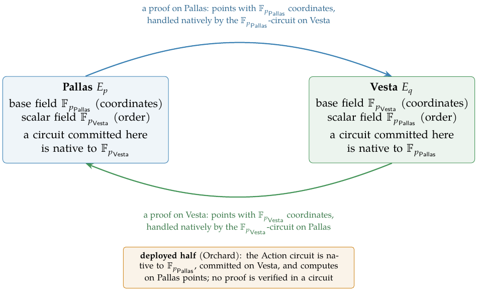
A curve $E$ over a prime field has two fields attached to it (Math Guide, §“Base fields, scalar fields, and the Pasta cycle”): the base field, in which its points’ coordinates lie and in which the group law’s slopes, squarings and inversions are computed, and the scalar field, the integers modulo the prime order of its group, in which the scalars of $[k]P$ live. Write $E_{p}$ for a curve over $\mathbb{F}_{p}$ and $q:=\#E_{p}(\mathbb{F}_{p})$ for its prime order, so that its base field is $\mathbb{F}_{p}$ and its scalar field $\mathbb{F}_{q}$ . A PLONKish circuit of Definition 2.7 is defined over one prime field $\mathbb{F}$ , its native field: its cells hold elements of $\mathbb{F}$ and its gates are polynomial identities over $\mathbb{F}$ , so an addition or multiplication in $\mathbb{F}$ costs one cell or one gate. Arithmetic in any other prime field is non-native: an element of the other field must be carried as several $\mathbb{F}$ -cells, each range-checked by the lookups of §2.7, and each of its operations becomes many gates with carries and reductions. Which field a circuit is native to is not a free choice. Its column polynomials are committed with the inner-product commitment of §3 on some curve, and a Pedersen commitment to a vector of $\mathbb{F}$ -elements needs a group whose scalar field is $\mathbb{F}$ ; so the native field of a circuit is the scalar field of the curve its proof is committed on, exactly as the Action circuit, native to $\mathbb{F}_{p_{\mathsf{Pallas}}}$ , is committed on Vesta, whose order is $p_{\mathsf{Pallas}}$ (§3.8).

Why one curve cannot host its own verifier.

Take a proof committed on $E_{p}$ . Its group elements, the column and quotient commitments, the cross terms $(L_{j},R_{j})$ and the deferred point of its opening, are points of $E_{p}$ with coordinates in $\mathbb{F}_{p}$ . The in-circuit folding of §7.3 adds and scales such points, which is base-field arithmetic in $\mathbb{F}_{p}$ , so a verifier circuit handles them natively only if its native field is $\mathbb{F}_{p}$ . But a circuit committed on $E_{p}$ is native to the scalar field $\mathbb{F}_{q}$ : its challenges, its structured scalars and every field operation of the succinct part are $\mathbb{F}_{q}$ -arithmetic. One curve would host both jobs only if $\mathbb{F}_{p}=\mathbb{F}_{q}$ , that is, $\#E_{p}(\mathbb{F}_{p})=p$ . Curves with exactly $p$ points exist; by Hasse’s theorem (Math Guide, §“The group structure of $E(\mathbb{F}_{p})$ ”), which writes $\#E_{p}(\mathbb{F}_{p})=p+1-t$ with the trace $t$ , they are the curves with $t=1$ , called anomalous. On an anomalous curve the discrete logarithm is computable in polynomial time, the attack of Smart, of Semaev and of Satoh and Araki, and the Crypto Guide lists “not anomalous” among the criteria a curve must meet to be used at all (§“Instantiation on elliptic curves; the Pasta curves”, the anti-Smart criterion). So no secure curve has $\mathbb{F}_{p}=\mathbb{F}_{q}$ , and no one curve can host both the coordinates of its proofs and its own verifier circuit natively.

The 2-cycle.

The efficient resolution uses two curves that trade fields. A 2-cycle of elliptic curves is a pair $(E_{p},E_{q})$ with

\#E_{p}(\mathbb{F}_{p})=q\qquad\text{and}\qquad\#E_{q}(\mathbb{F}_{q})=p,

both primes: the scalar field of each curve is the base field of the other. Then:

1.

a circuit committed on $E_{q}$ has native field $\mathbb{F}_{p}$ , the scalar field of $E_{q}$ ; and $\mathbb{F}_{p}$ is the coordinate field of $E_{p}$ , so that circuit manipulates the points of a proof produced over $E_{p}$ natively, and verifies such a proof at the cost §7.3 counted, the proof’s scalars aside;
2.

the proof that circuit produces is committed on $E_{q}$ , and its points have coordinates in $\mathbb{F}_{q}$ , the native field of a circuit committed on $E_{p}$ ; so a circuit over $\mathbb{F}_{q}$ handles its points natively in turn;
3.

the proofs of a chain alternate between the two curves, each step handling its predecessor’s points natively (Figure 20).

What the cycle does and does not buy.

The cycle makes the preceding curve’s coordinate arithmetic native; it does not identify the two scalar fields, which remain distinct primes. Challenges squeezed in the previous proof’s field and the scalars derived from them are $\mathbb{F}_{p}$ -elements that the $\mathbb{F}_{q}$ -native circuit must handle: they need compatible encodings across the two fields, range checks where an element of the larger field is carried in the smaller, and, where a genuine $\mathbb{F}_{p}$ multiplication is unavoidable, non-native scalar arithmetic. Nor is the cycle a logical necessity. A single curve could verify its own proofs with non-native coordinate arithmetic throughout, at a cost of many gates per point operation multiplied by the $O(\log d)$ point operations of the succinct part; that is possible and substantially more expensive. The cycle is the efficient native design, not the only correct one.

The deployed instance.

The Pasta cycle of the Math Guide (§“Base fields, scalar fields, and the Pasta cycle”; §“Pallas and Vesta assembled”) is a 2-cycle: Pallas is defined over $\mathbb{F}_{p_{\mathsf{Pallas}}}$ with group order $p_{\mathsf{Vesta}}$ , and Vesta over $\mathbb{F}_{p_{\mathsf{Vesta}}}$ with group order $p_{\mathsf{Pallas}}$ , both curves $y^{2}=x^{3}+5$ (protocol specification, § 5.4.9.6, “Pallas and Vesta”). The cycle follows from the specification’s two primes and nothing else. With

	$\displaystyle p_{\mathsf{Pallas}}$	$\displaystyle=\mathtt{0x40000000\,00000000\,00000000\,00000000\,224698fc\,094% cf91b\,992d30ed\,00000001},$
	$\displaystyle p_{\mathsf{Vesta}}$	$\displaystyle=\mathtt{0x40000000\,00000000\,00000000\,00000000\,224698fc\,0994% a8dd\,8c46eb21\,00000001},$

the point $(-1,2)$ lies on Pallas, $[p_{\mathsf{Vesta}}]\,(-1,2)=\mathcal{O}$ there, and exactly one multiple of $p_{\mathsf{Vesta}}$ lies in the Hasse interval $[\,p+1-2\sqrt{p},\;p+1+2\sqrt{p}\,]$ for $p=p_{\mathsf{Pallas}}$ . That settles the order: the order of the point $(-1,2)$ divides the prime $p_{\mathsf{Vesta}}$ and is not $1$ , so it is $p_{\mathsf{Vesta}}$ , which therefore divides $\#\mathcal{E}(\mathbb{F}_{p_{\mathsf{Pallas}}})$ by Lagrange’s theorem (Math Guide, §“Cosets and Lagrange’s theorem”); the group order lies in an interval of length $4\sqrt{p}$ , far shorter than $p_{\mathsf{Vesta}}$ , which contains one multiple of $p_{\mathsf{Vesta}}$ ; hence $\#\mathcal{E}(\mathbb{F}_{p_{\mathsf{Pallas}}})=p_{\mathsf{Vesta}}$ . The symmetric check on Vesta shows that the Vesta group has order $p_{\mathsf{Pallas}}$ . The traces are

	$\displaystyle t_{\mathsf{Pallas}}$	$\displaystyle=p_{\mathsf{Pallas}}+1-p_{\mathsf{Vesta}}=-8666372506598404339531% 7759,$
	$\displaystyle t_{\mathsf{Vesta}}$	$\displaystyle=p_{\mathsf{Vesta}}+1-p_{\mathsf{Pallas}}=86663725065984043395317% 761,$

each far inside the Hasse bound and neither equal to $1$ : neither curve is anomalous, as the Crypto Guide’s criterion requires. The two traces sum to $2$ , as they must for any 2-cycle, since $(p+1-q)+(q+1-p)=2$ ; the toy curve of §3.7, $y^{2}=x^{3}+3$ over $\mathbb{F}_{79}$ with $97$ points, has trace $79+1-97=-17$ , and the case excluded in that subsection, a curve over $\mathbb{F}_{97}$ with $97$ points and so trace $1$ , is exactly the anomalous one.

The cycle in the accumulation chain.

The Pasta cycle renders each step of §7.3 native. A proof committed on Vesta is produced by a circuit native to $\mathbb{F}_{p_{\mathsf{Pallas}}}$ ; that circuit verifies the previous proof of the chain, committed on Pallas, whose group elements, the column and quotient commitments, the pairs $(L_{j},R_{j})$ and the point of the Pallas accumulator instance it forwards, have coordinates in exactly $\mathbb{F}_{p_{\mathsf{Pallas}}}$ , so the point arithmetic of the succinct checks and of the fold (36) is native. The next proof, committed on Pallas by a circuit native to $\mathbb{F}_{p_{\mathsf{Vesta}}}$ , verifies the Vesta proof by the symmetric argument. This cross-curve alternation avoids non-native emulation of the preceding curve’s coordinate field; as “What the cycle does and does not buy” said, it does not eliminate the scalar-field conversions.

The half Orchard uses.

This is the part of the cycle in consensus. The Action circuit is native to $\mathbb{F}_{p_{\mathsf{Pallas}}}$ and committed on Vesta (§3.8), and the statement it proves manipulates Pallas points: the note commitment $\mathsf{cm}$ , a Pallas point whose $x$ -coordinate $\mathsf{cmx}$ is a public input; the randomised verification key $\mathsf{rk}$ ; and the net value commitment $\mathsf{cv}^{\mathrm{net}}$ , the last two exposed by their coordinates in the instance column of §4.2. Their coordinates lie in $\mathbb{F}_{p_{\mathsf{Pallas}}}$ , the circuit’s native field, by the very coincidence the cycle is built on, so the circuit computes on them natively, with gates such as the incomplete-addition gate of §4.1.2. The protocol specification records the arrangement: Vesta for the proof system, Pallas for the application circuit, both curves designed to be efficiently implementable inside a circuit though only Pallas is so used (protocol specification, § 5.4.9.6, “Pallas and Vesta”); ZIP 224 says the same in the language of this subsection, that the proposal uses half of the cycle, Pallas being the curve embedded in Vesta’s circuits, and that the full cycle is left for future use (ZIP 224, under “Curves”). One direction of Figure 20 is thus in consensus today; the return arrow, and everything in this section that depends on it, is not.