The Zcash ArboretumI–IX The Complete Arboretum
Contents
PDF
Theme

11 Probability, asymptotics, and computation

This section fixes the language of security claims: probability, asymptotic notation, and efficient computation. It proves the union and birthday bounds, the properties of statistical distance, the bias bound for modular reduction, Wald’s identity, Chernoff bounds for the arrival counts of exponential clocks, and the closure of negligible functions under addition and multiplication by polynomials. The birthday bound sets hash output lengths, and the bias bound justifies the sampling of Orchard scalars; later volumes build their block-discovery and extraction analyses on the waiting-time and clock results. A signature scheme advertised as offering “128-bit security” cannot exclude forgery: a forger that guesses the secret key, a finite string, succeeds with positive probability, so the claim bounds the success probability of every attacker within stated resources; §11.11 states what it asserts. Probability spaces are finite until §11.7; finite spaces suffice for keys, bounded-length messages, group elements, and the coins of an algorithm with a fixed running-time bound. The prerequisites are finite sets, sums, and elementary calculus: limits, the exponential function, and, for the density-defined laws of §11.7, the improper Riemann integral.

11.1 Finite probability spaces and events

Definition 11.1 (Finite probability space).

A finite probability space is a pair (Ω,Pr) where Ω is a nonempty finite set, called the sample space, and Pr:Ω→[0,1] is a function, called the probability mass function, satisfying the normalisation condition

∑ω∈ΩPr⁡[ω]=1.

An element ω∈Ω is an outcome (or elementary event).

Definition 11.2 (Event).

An event is a subset A⊆Ω. Its probability is

Pr⁡[A]=∑ω∈APr⁡[ω],

with the convention Pr[∅]=0 (an empty sum). The event A occurs on outcome ω if ω∈A.

Because Ω is finite, every subset is an event. On an uncountable sample space the general theory specifies a family of admissible events together with its probability assignment; Remark 11.31 marks the one place this series requires measure theory. The following facts are used without further citation.

Proposition 11.3 (Basic axioms).

For any finite probability space (Ω,Pr) and events A,B⊆Ω:

  1. 1.

    0≤Pr[A]≤1, Pr[∅]=0, and Pr[Ω]=1.

  2. 2.

    (Complement.) Pr[Ω∖A]=1−Pr[A].

  3. 3.

    (Monotonicity.) If A⊆B then Pr[A]≤Pr[B].

  4. 4.

    (Inclusion–exclusion for two events.) Pr[A∪B]=Pr[A]+Pr[B]−Pr[A∩B].

  5. 5.

    (Finite additivity.) If A1,…,An are pairwise disjoint then Pr[⋃i=1nAi]=∑i=1nPr[Ai].

Proof.

Every claim follows by manipulating the defining sums. For (1), each summand Pr[ω] lies in [0,1] and the total is 1 by normalisation; an event’s probability is a partial sum of nonnegative terms, hence lies in [0,1]. For (2), the sets A and Ω∖A partition Ω, so Pr[A]+Pr[Ω∖A]=∑ω∈ΩPr[ω]=1. For (3), splitting the sum over B gives Pr[B]=∑ω∈APr[ω]+∑ω∈B∖APr[ω]≥Pr[A], the second term being a sum of nonnegative numbers. For (5), disjointness means each ω in the union lies in exactly one Ai, so the double sum ∑i∑ω∈AiPr[ω] counts each ω∈⋃iAi exactly once. For (4), write A∪B=A⊔(B∖A) (disjoint), so by (5) Pr[A∪B]=Pr[A]+Pr[B∖A]; also B=(A∩B)⊔(B∖A), giving Pr[B∖A]=Pr[B]−Pr[A∩B]. Substituting yields the claim. □

The distribution used most often in cryptography is the uniform distribution.

Definition 11.4 (Uniform distribution).

Let S be a nonempty finite set. The uniform distribution on S is the probability space (S,Pr) with Pr[ω]=1/|S| for every ω∈S. The notation x←S (or x←$S) means that x is sampled according to the uniform distribution on S. Under the uniform distribution, for any event A⊆S,

Pr⁡[A]=|A||S|.

11.2 Conditional probability and independence

Conditioning updates the probability of one event on the information that another has occurred.

Definition 11.5 (Conditional probability).

Let A,B be events with Pr[B]>0. The conditional probability of A given B is

Pr⁡[A∣B]=Pr⁡[A∩B]Pr⁡[B].

When Pr[B]=0 the quantity is left undefined.

Conditioning on B restricts the sample space to B and renormalises so that B has probability 1: the map ω↦Pr[{ω}∣B] is itself a probability mass function on B, and Pr[A∣B] is the probability it assigns to A∩B.

Proposition 11.6 (Chain rule and total probability).

Let A1,…,An be events with Pr[A1∩⋯∩An−1]>0. Then

Pr⁡[A1∩⋯∩An]=Pr⁡[A1]⁢Pr⁡[A2∣A1]⁢Pr⁡[A3∣A1∩A2]⁢⋯⁢Pr⁡[An∣A1∩⋯∩An−1].

Moreover, if B1,…,Bk partition Ω (pairwise disjoint with union Ω) and each Pr[Bi]>0, then for any event A,

Pr⁡[A]=∑i=1kPr⁡[A∣Bi]⁢Pr⁡[Bi].
Proof.

The chain rule follows by telescoping: each factor Pr[Aj∣A1∩⋯∩Aj−1] equals Pr[A1∩⋯∩Aj]/Pr[A1∩⋯∩Aj−1] by 11.5, and the product collapses to Pr[A1∩⋯∩An]/1. (Monotonicity ensures that all the intermediate intersections have positive probability, so every factor is defined.) For total probability, the events A∩Bi are pairwise disjoint with union A (since the Bi partition Ω), so finite additivity and Pr[A∩Bi]=Pr[A∣Bi]Pr[Bi] give Pr[A]=∑iPr[A∩Bi]=∑iPr[A∣Bi]Pr[Bi]. □

Independence is the formal statement that one event carries no information about another.

Definition 11.7 (Independence of events).

Two events A,B are independent if

Pr⁡[A∩B]=Pr⁡[A]⁢Pr⁡[B].

A family {Ai}i∈I of events is mutually independent if for every finite subset J⊆I,

Pr⁡[⋂i∈JAi]=∏i∈JPr⁡[Ai].
Remark 11.8.

When Pr[B]>0, independence of A and B is equivalent to Pr[A∣B]=Pr[A]. Mutual independence is strictly stronger than pairwise independence. The standard counterexample consists of two fair coin tosses, with A “the first is heads”, B “the second is heads”, and C “the two coins differ”. Each pair is independent, yet Pr[A∩B∩C]=0≠18=Pr[A]Pr[B]Pr[C], so the three are not mutually independent.

11.3 Random variables and expectation

Definition 11.9 (Random variable).

Let (Ω,Pr) be a finite probability space and T any set. A (T-valued) random variable is a function X:Ω→T. When T⊆ℝ, we call X real-valued. For t∈T,

Pr⁡[X=t]=Pr⁡[{ω∈Ω:X⁢(ω)=t}],

and more generally Pr[X∈B] denotes the probability that X takes a value in B⊆T. The function t↦Pr[X=t] on the finite image of X is the distribution (or law) of X.

Definition 11.10 (Independent random variables).

Random variables X1,…,Xn (with values in sets T1,…,Tn) are mutually independent if for all t1∈T1,…,tn∈Tn,

Pr⁡[X1=t1,…,Xn=tn]=∏i=1nPr⁡[Xi=ti].
Definition 11.11 (Expectation).

Let X:Ω→ℝ be a real-valued random variable on a finite space. Its expectation (or mean) is

𝔼⁢[X]=∑ω∈ΩX⁢(ω)⁢Pr⁡[ω]=∑t∈im⁡(X)t⋅Pr⁡[X=t],

where im(X) denotes the (finite) image of X. The two expressions agree by grouping outcomes according to their X-value.

Definition 11.12 (Indicator).

For an event A, its indicator random variable 𝟏A:Ω→{0,1} takes the value 𝟏A(ω)=1 if ω∈A and 0 otherwise.

Proposition 11.13 (Indicator expectation).

For any event A, 𝔼[𝟏A]=Pr[A].

Proof.

By 11.11, 𝔼[𝟏A]=∑ω𝟏A(ω)Pr[ω]=∑ω∈APr[ω]=Pr[A], since the indicator vanishes off A. □

Theorem 11.14 (Linearity of expectation).

Let X,Y:Ω→ℝ be random variables on a finite space and a,b∈ℝ. Then

𝔼⁢[a⁢X+b⁢Y]=a⁢𝔼⁢[X]+b⁢𝔼⁢[Y].

More generally, for random variables X1,…,Xn and scalars a1,…,an,

𝔼⁢[∑i=1nai⁢Xi]=∑i=1nai⁢𝔼⁢[Xi].

This holds whether or not the Xi are independent.

Proof.

Directly from the definition,

𝔼⁢[a⁢X+b⁢Y] =∑ω∈Ω(a⁢X⁢(ω)+b⁢Y⁢(ω))⁢Pr⁡[ω]
=a⁢∑ωX⁢(ω)⁢Pr⁡[ω]+b⁢∑ωY⁢(ω)⁢Pr⁡[ω]
=a⁢𝔼⁢[X]+b⁢𝔼⁢[Y],

splitting the finite sum and extracting the constants. The n-term statement follows by induction on n. □

The following consequence underlies every averaging (“heavy-row”) argument in the series.

Proposition 11.15 (Markov’s inequality).

Let X≥0 be a real-valued random variable and a>0. Then Pr[X≥a]≤𝔼[X]/a.

Proof.

Every outcome contributes nonnegatively to 𝔼[X], and each outcome with X(ω)≥a contributes at least aPr[ω]; hence 𝔼[X]≥aPr[X≥a]. □

11.4 The union bound and a birthday calculation

This subsection proves the union bound, the inequality used most often in cryptographic proofs; it requires no independence. It gives the upper half of the birthday bound, which governs how soon collisions appear under uniform sampling: among roughly N uniform samples from a set of size N, two are likely to coincide. The birthday bound sets the output lengths of cryptographic hash functions.

Theorem 11.16 (Union bound / Boole’s inequality).

For any events A1,…,An in a finite probability space,

Pr⁡[⋃i=1nAi]≤∑i=1nPr⁡[Ai].
Proof.

Disjointify the union into “first occurrence” events: B1=A1 and Bi=Ai∖(A1∪⋯∪Ai−1) for i≥2. The Bi are pairwise disjoint, Bi⊆Ai, and ⋃iBi=⋃iAi. By finite additivity and monotonicity (11.3),

Pr⁡[⋃iAi]=Pr⁡[⋃iBi]=∑iPr⁡[Bi]≤∑iPr⁡[Ai].∎

The “first occurrence” disjointification recurs, in a telescoping form for increasing chains, in the proof of the continuity theorem of §11.7. Taking complements in the union bound gives the corresponding inequality for conjunctions.

Corollary 11.17 (Union bound for the good event).

If each event Ai holds except with probability at most εi (that is, Pr[Ω∖Ai]≤εi), then all of them hold simultaneously except with probability at most ∑iεi:

Pr⁡[⋂i=1nAi]≥1−∑i=1nεi.
Proof.

By De Morgan, Ω∖⋂iAi=⋃i(Ω∖Ai). Apply the union bound to the complements and take the complement of both sides. □

Proposition 11.18 (Birthday bound).

Sample x1,…,xk independently and uniformly from a set of size N, and let C be the event that some two of them collide, i.e. xi=xj for some i<j. Then

Pr⁡[C]≤(k2)⁢1N=k⁢(k−1)2⁢N,

and, on the other side,

Pr⁡[C]=1−∏i=0k−1(1−iN)≥1−e−k⁢(k−1)/(2⁢N).

In particular a collision becomes likely once k=Θ(N).

Proof.

Upper bound. For i<j let Ai⁢j be the event xi=xj. Since xi and xj are independent and uniform, Pr[Ai⁢j]=∑vPr[xi=v]Pr[xj=v]=N⋅(1/N)2=1/N. Now C=⋃i<jAi⁢j, a union of (k2) events, one per two-element subset of the indices (6.13), so the union bound (11.16) gives Pr[C]≤(k2)/N.

Lower bound. The complement C¯ is the event that all k samples are distinct. If k>N, the pigeonhole principle forces a collision, so Pr[C¯]=0; the product also vanishes, through its factor 1−N/N, so the stated equality holds and the exponential bound is trivial. Let then k≤N, and for 0≤i≤k let Di be the event that the first i samples are pairwise distinct (D0=D1=Ω, and Dk=C¯). We show Pr[Di]=∏j=0i−1(1−j/N) by induction on i≤k; every factor is positive, since j≤k−1≤N−1, so in particular each Di has positive probability and conditioning on it is legitimate (11.5). For the step, the events pinning the first i samples to specific distinct values partition Di, each with probability N−i>0 by independence and uniformity; given any one of them, the next sample avoids the i values taken with probability 1−i/N, again by independence and uniformity. Averaging over the cells (total probability, 11.6) gives Pr[Di+1∣Di]=1−i/N, and Pr[Di+1]=Pr[Di+1∣Di]Pr[Di] completes the induction. Taking i=k yields the stated equality, in which every factor is nonnegative, so the inequality 1−x≤e−x applies factor by factor. (For 0≤x<1 this inequality follows from Bernoulli’s inequality, (1−x/n)n≥1−x for n>x, by letting n→∞ in the limit definition of e−x; for x≥1 the left side is nonpositive.) Thus

Pr⁡[C¯]=∏i=0k−1(1−iN)≤∏i=0k−1e−i/N=exp⁡(−1N⁢∑i=0k−1i)=e−k⁢(k−1)/(2⁢N),

summing the exponents via ∑i=0k−1i=k(k−1)/2. Taking complements gives Pr[C]=1−Pr[C¯]≥1−e−k⁢(k−1)/(2⁢N). □

Example 11.19.

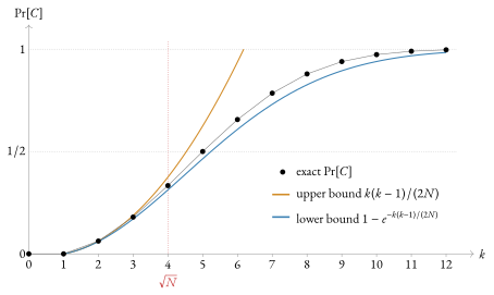
With N=365 and k=23, the classical birthday problem, the exact product gives Pr[C]=0.5073, a probability above one half, and the proposition brackets it as 0.5000≤Pr[C]≤0.6932. The threshold appears at small scale as well: with N=16, the fifth sample, the first beyond 16=4, raises the collision probability above one half, Pr[C]=0.5001 at k=5. 7 plots the exact probability and both bounds for N=16.

Refer to caption
Figure 7: The collision probability Pr[C] of 11.18 for N=16, against the sample count k: the exact value at each k, with the upper and lower bounds of the proposition. The upper bound exceeds 1, and so says nothing, from k=7 on. At k=5, the first count beyond the threshold N=4, the exact probability passes one half (11.19).
Remark 11.20.

The threshold k≈N is the reason an n-bit hash function (so N=2n) offers only about 2n/2 collision resistance: an adversary expects a collision after roughly 2n/2 random evaluations — for N=2256, that is 2256=2128. Output lengths are therefore chosen twice the desired security level. The same square-root phenomenon recurs in random-walk discrete-log attacks (Pollard’s rho, 10.30), so the curves used in Halo 2 and Orchard are sized so that N itself lies far beyond feasible computation.

11.5 Statistical distance

Statistical distance measures how far apart two distributions are, such as a real key-generation procedure and an idealised uniform one; it formalises “no statistical test can distinguish them well”.

Definition 11.21 (Statistical distance).

Let P and Q be probability distributions on the same finite set S (i.e. probability mass functions P,Q:S→[0,1]). Their statistical distance (or total variation distance) is

Δ⁢(P,Q)=12⁢∑s∈S|P⁢(s)−Q⁢(s)|.

For random variables X,Y with values in S, Δ(X,Y) denotes the statistical distance of their distributions.

The factor 12 makes Δ range over [0,1] and makes it equal to the maximum advantage of a distinguisher, as part (3) of the next theorem establishes.

Theorem 11.22 (Properties of statistical distance).

Let P,Q,R be distributions on a finite set S. Then:

  1. 1.

    0≤Δ(P,Q)≤1; and Δ(P,Q)=0 if and only if P=Q.

  2. 2.

    (Metric.) Δ is symmetric and satisfies the triangle inequality Δ(P,R)≤Δ(P,Q)+Δ(Q,R).

  3. 3.

    (Variational characterisation.) Δ(P,Q)=maxA⊆S(P(A)−Q(A))=maxA⊆S|P(A)−Q(A)|, where P(A)=∑s∈AP(s).

  4. 4.

    (Data processing / post-processing.) For any (possibly randomised) function f applied to a sample, Δ(f(P),f(Q))≤Δ(P,Q). In particular no algorithm can increase statistical distance.

Proof.

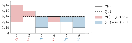
(1) Nonnegativity holds termwise. For the upper bound, split S into S+={s:P(s)≥Q(s)} and S−=S∖S+. Since ∑sP(s)=∑sQ(s)=1, we have ∑s(P(s)−Q(s))=0, so ∑s∈S+(P(s)−Q(s))=∑s∈S−(Q(s)−P(s))=:D≥0. Hence Δ(P,Q)=12(∑S+(P−Q)+∑S−(Q−P))=D. 8 draws the two sums as equal areas. As D=∑S+(P(s)−Q(s))≤∑S+P(s)≤1, we get Δ≤1. If Δ=0 then every |P(s)−Q(s)|=0, so P=Q; the converse is immediate.

(2) Symmetry holds termwise. For the triangle inequality, |P(s)−R(s)|≤|P(s)−Q(s)|+|Q(s)−R(s)| termwise by the triangle inequality on ℝ; summing over s and halving gives the claim.

(3) With D as above, take A=S+: then P(A)−Q(A)=∑S+(P−Q)=D=Δ(P,Q), so the maximum is at least Δ. Conversely, for any A⊆S, P(A)−Q(A)=∑s∈A(P(s)−Q(s))≤∑s∈A∩S+(P(s)−Q(s))≤D=Δ, since dropping the negative terms only increases the sum and extending from A∩S+ to all of S+ increases it further. Thus the maximum over A of P(A)−Q(A) is exactly Δ; replacing A by its complement swaps the sign, giving the same value for maxA|P(A)−Q(A)|.

(4) First take f deterministic, f:S→U. For u∈U, f(P)(u)=P(f−1(u)). Then

Δ⁢(f⁢(P),f⁢(Q))=12⁢∑u|P⁢(f−1⁢(u))−Q⁢(f−1⁢(u))|≤12⁢∑u∑s∈f−1⁢(u)|P⁢(s)−Q⁢(s)|=Δ⁢(P,Q),

using |∑sas|≤∑s|as| on each fibre, and that the fibres f−1(u) partition S. A randomised f is a deterministic function of the sample s together with independent fresh coins r; apply the deterministic case to the joint variable (s,r), noting that the two joint distributions P×Ur and Q×Ur have the same statistical distance Δ(P,Q), the shared coin distribution contributing nothing. □

Refer to caption
Figure 8: Statistical distance as area, for the distributions P=(5,4,1,3,2,1)/16 and Q=(2,3,3,2,3,3)/16 on S={1,…,6}, drawn as overlaid bar charts of unit width. The shading between the two bar heights has total area ∑s|P(s)−Q(s)|=10/16. Its part over S+={1,2,4}, where P exceeds Q, and its part over S−={3,5,6} each have area 5/16, and Δ(P,Q)=5/16 is half the total.
Remark 11.23 (Distinguishing interpretation).

Part (3) states that Δ(P,Q) is exactly the best advantage of any test — even a computationally unbounded one — that, given a single sample, must guess whether it came from P or Q: the optimal test outputs “P” on the set A=S+, and its advantage PrP[A]−PrQ[A] equals Δ(P,Q). Part (4) makes statistical distance compose in proofs: if Δ(P,Q)≤ε, then P and Q are interchangeable in any analysis at the cost of an additive ε in every probability. When ε is negligible (11.61 below), we call P and Q statistically indistinguishable.

11.6 Uniform sampling and the bias of modular reduction

The most tractable source of randomness is a stream of independent uniform bits, whereas cryptography requires uniform elements of other finite sets: a scalar in ℤ/qℤ (2), a field element of 𝔽p (6), a point in a group. If the target set S has |S|=2ℓ, reading ℓ uniform bits as a number in {0,…,2ℓ−1} and indexing into S is exact. When |S| is not a power of two — most importantly when S=ℤ/qℤ for a prime q, the scalar field of an elliptic curve (10) — a common method is reduce-modulo: sample a long uniform integer and reduce it mod q. Some residues then receive one more preimage than others; the next proposition bounds the resulting bias.

Proposition 11.24 (Bias of modular reduction).

Let q≥2 be an integer and let K=2L for a nonnegative integer L. Sample U uniformly from {0,1,…,K−1} (equivalently, read L uniform bits as an integer), and set R=Umodq∈{0,1,…,q−1}. Let 𝒰q denote the uniform distribution on {0,…,q−1}. Then the statistical distance of R from uniform satisfies

Δ⁢(R,𝒰q)≤qK=q2L.

Consequently, if q<2n and one takes L=n+s bits, then Δ(R,𝒰q)<2−s.

Proof.

Write K=mq+t with m=⌊K/q⌋ and remainder t=Kmodq, so 0≤t<q. For a residue r∈{0,…,q−1}, the number of integers in {0,…,K−1} congruent to r modulo q is m+1 if r<t and m if r≥t. Hence

Pr⁡[R=r]={(m+1)/K,r<t,m/K,r≥t.

Comparing with the target probability 1/q and using m/K≤1/q≤(m+1)/K (since mq≤K≤(m+1)q),

|Pr⁡[R=r]−1q|≤m+1K−mK=1Kfor every ⁢r.

Therefore

Δ⁢(R,𝒰q)=12⁢∑r=0q−1|Pr⁡[R=r]−1q|≤12⋅q⋅1K=q2⁢K≤qK.

(The computation yields the sharper bound q/(2K); q/K is the usual stated form.) For the final claim, q<2n and K=2n+s give q/K<2n/2n+s=2−s. □

Example 11.25.

Let L=6 uniform bits be reduced modulo q=5. Then K=64=12⋅5+4, so the four residues r<4 receive 13 preimages each and the residue r=4 receives 12; the statistical distance from uniform is exactly 1/80, within the guarantee 2−3 of the proposition (as q<23 and s=6−3=3).

Remark 11.26 (Sampling scalars in practice).

By the proposition, a scalar modulo a ∼256-bit prime q with statistical distance below 2−128 from uniform is obtained by reducing 256+128=384 uniform bits modulo q. The bias 2−s, with the slack s set to the security parameter, is negligible (11.61), so the reduce-modulo sample is statistically indistinguishable from a perfectly uniform scalar, and by the data-processing inequality (11.22(4)) substituting one for the other anywhere costs at most 2−128 per use. An alternative, rejection sampling, draws ⌈log2q⌉ bits, accepts if the result is <q, and otherwise retries; it gives exactly uniform output at the cost of a variable but (with overwhelming probability) small number of retries. For this series the negligible bias of reduce-modulo is acceptable and simpler to analyse. The Orchard specification employs this reduce-modulo sampling when deriving scalars from hash outputs: its ToScalar reduces the full 512-bit 𝖯𝖱𝖥𝖾𝗑𝗉𝖺𝗇𝖽 output modulo the 255-bit group order, a slack of 257 bits, well beyond the 128-bit slack computed above (Zcash protocol specification §4.2.3 and §5.4.2).

11.7 Beyond finite spaces: countable additivity, limits, and densities

Two uses require more than a finite sample space. A process observed until an event occurs, such as an unbounded retry loop or a random walk run until it first hits a barrier, has no finite horizon, even when it terminates with probability one; a waiting time measured in continuous units has no finite sample space. This subsection adds countable additivity, continuity along monotone events, and laws defined by densities, and states in Remark 11.31 the measure-theoretic results it assumes.

Definition 11.27 (Countable probability space).

A countable probability space is a pair (Ω,Pr) in which Ω is a countable set and Pr:Ω→[0,1] satisfies ∑ω∈ΩPr[ω]=1; the sum is independent of the enumeration order because its terms are nonnegative. Events are arbitrary subsets A⊆Ω, with Pr[A]=∑ω∈APr[ω], and Definitions 11.2–11.11 carry over with “finite” read as “countable” (a random variable’s image may now be countably infinite), with one exception: 11.4 does not — equal weights cannot sum to 1 on a countably infinite set, so the uniform distribution remains a strictly finite notion. Expectation additionally requires its defining sum to converge absolutely.

Proposition 11.28 (Countable additivity).

Let (Ω,Pr) be a countable probability space and A1,A2,… pairwise disjoint events. Then

Pr⁡[⋃n≥1An]=∑n≥1Pr⁡[An],

and in particular the basic axioms of 11.3 hold unchanged.

Proof.

Every outcome of the union lies in exactly one An, so both sides sum the same nonnegative terms Pr[ω], grouped differently; a series of nonnegative terms may be summed in any order, or in groups, without changing its value. □

Theorem 11.29 (Continuity along monotone events).

Let Pr be a probability assignment, on any sample space, defined for a family of events closed under complement and countable union, and countably additive on it. If A1⊆A2⊆⋯ is an increasing chain of events, then

Pr⁡[⋃n≥1An]=limn→∞Pr⁡[An],

and dually Pr[⋂nBn]=limnPr[Bn] for a decreasing chain B1⊇B2⊇⋯. On a countable space the hypothesis holds automatically, by 11.28.

Proof.

Disjointify by telescoping: set D1=A1 and Dn=An∖An−1 for n≥2. The Dn are pairwise disjoint, ⋃k≤nDk=An, and ⋃nDn=⋃nAn. Countable additivity gives

Pr⁡[⋃nAn]=∑n≥1Pr⁡[Dn]=limn→∞∑k=1nPr⁡[Dk]=limn→∞Pr⁡[An],

the final step by finite additivity. The decreasing case follows by complementation. □

Definition 11.30 (Infinite sequence of independent trials).

Fix a finite outcome set T and a distribution p on T. An infinite sequence of independent trials with law p is a sequence of random variables X1,X2,… such that every prefix (X1,…,Xn) consists of n mutually independent p-distributed trials in the sense of 11.10 — equivalently, the prefix’s law is that of the finite probability space Tn carrying the product weights Pr[(t1,…,tn)]=p(t1)⋯p(tn). An event is finitely determined if membership in it is decided by some fixed finite prefix; its probability is the finite-space value. An event of the form “some prefix satisfies P” is the union of an increasing chain of finitely determined events, and 11.29 assigns it the limit of the prefix probabilities.

Remark 11.31 (Assumed measure-theoretic results).

11.30 presumes that a single, countably additive probability assignment on infinite sequences exists that restricts correctly to every finite prefix at once. That existence statement is the Kolmogorov extension theorem, and its proof belongs to measure theory, which lies off this series’ critical path: the space of infinite sequences over at least two possible outcomes is uncountable, so it escapes 11.27, and the extension specifies the admissible events. This series therefore takes it, with its countable additivity and hence 11.29, as an assumption rather than a theorem. On infinite-sequence spaces, only finitely determined events and their monotone limits appear in this series, and for those the values are determined by the finite theory together with continuity; the density-defined laws of 11.32 rest on the analogous assumption, their interval and joint-event probabilities being taken to cohere as the stated integrals. The independent families of 11.40 extend that assumption in two ways: joint events of several density-defined quantities are taken to be iterated integrals, in whichever order of integration is convenient — the exchange of order for nonnegative integrands is the Fubini–Tonelli theorem, likewise measure-theoretic — and the gap sequences of 11.44 are infinite families, of which only finite prefixes enter any event this series uses, except through countable unions over the values of an arrival count — N(t) of 11.44, or the count X of 11.51, each event “count =x” being a joint event of finitely many gaps. For any set B of values, the event “count ∈B” — among them the event that the count is finite, and the tail events of 11.49 — is taken to have probability ∑x∈BPr[count=x], by the countable additivity assumed above.

Definition 11.32 (Law defined by a density).

A real-valued random quantity X has density f:ℝ→ℝ≥0 if ∫−∞∞f(t)𝑑t=1 and

Pr⁡[a≤X≤b]=∫abf⁢(t)⁢𝑑tfor all ⁢a≤b;

improper Riemann integrals suffice throughout this series. The distribution function is F(t)=Pr[X≤t]=∫−∞tf, so Pr[X>t]=1−F(t), and single points carry probability zero. The expectation is 𝔼[X]=∫−∞∞tf(t)𝑑t when this integral converges absolutely. Two density-defined quantities X,Y are independent if Pr[X∈I,Y∈J]=Pr[X∈I]Pr[Y∈J] for all intervals I,J; probabilities of joint events are then taken to factor through iterated integrals of the product fX(s)fY(t).

11.7.1 Waiting times: tail sums, geometric trials, and Wald’s identity

The results of this unit need only countable expectation and finitely determined events. For a variable with values in ℕ∪{∞}, the defining sum of the expectation has nonnegative terms, and the value +∞ is permitted when it diverges.

Lemma 11.33 (Tail-sum formula).

Let T be a random variable with values in ℕ∪{∞} and Pr[T=∞]=0. Then 𝔼[T]=∑k≥1Pr[T≥k], either side being infinite exactly when the other is.

Proof.

Expanding Pr[T≥k]=∑m≥kPr[T=m] and regrouping the doubly indexed nonnegative series, each term Pr[T=m] is counted once for every k≤m, that is, m times; nonnegative series may be regrouped freely. □

Proposition 11.34 (Geometric waiting time).

In an infinite sequence of independent trials, each succeeding with probability ε>0, let T be the index of the first success. Then Pr[T≥k]=(1−ε)k−1 and 𝔼[T]=1/ε.

Proof.

The event T≥k says the first k−1 trials all fail — a finitely determined event of probability (1−ε)k−1; in particular Pr[T=∞]=limk(1−ε)k−1=0 by continuity (11.29). The tail-sum formula then gives 𝔼[T]=∑k≥1(1−ε)k−1=1/ε, a geometric series. □

Proposition 11.35 (Wald’s identity).

Let X1,X2,… be an infinite sequence of independent trials with common law, each Xi≥0 with finite mean, and let T be a stopping rule: a random index such that, for every k, whether T=k is decided by the first k trials alone. If 𝔼[T]<∞, then

𝔼⁢[∑i=1TXi]=𝔼⁢[T]⋅𝔼⁢[X1].
Proof.

Write S=∑i=1TXi and Sk=∑i=1kXi, so that S=Sk on the event T=k. The hypothesis 𝔼[T]<∞ forces Pr[T=∞]=0, by the convention preceding 11.33. The variable S takes countably many values — on {T=k} it agrees with Sk, whose values run over a finite set, the trials having finitely many outcomes — and each event {S=s} is the disjoint countable union ⋃k{T=k,Sk=s} of finitely determined events, so its probability is assigned by countable additivity (11.31). By 𝔼[S] we mean ∑ssPr[S=s], the expectation of this countably supported distribution, a sum of nonnegative terms.

Expanding each Pr[S=s] and regrouping the doubly indexed nonnegative series,

𝔼⁢[S]=∑ss⁢∑k≥1Pr⁡[T=k,Sk=s]=∑k≥1𝔼⁢[Sk⁢𝟏T=k],

each inner expectation living on the finite prefix space of the first k trials (11.30), where linearity (11.14) expands it as ∑i=1k𝔼[Xi𝟏T=k]. Regrouping the nonnegative double series once more,

𝔼⁢[S]=∑i≥1∑k≥i𝔼⁢[Xi⁢𝟏T=k].

Fix i and let n≥i. The events T=k (for k≤n), T>n, and T≥i are all decided by the first n trials, and on that prefix space the pointwise identity 𝟏T≥i=∑k=in𝟏T=k+𝟏T>n holds, so linearity gives

∑k=in𝔼⁢[Xi⁢𝟏T=k]=𝔼⁢[Xi⁢𝟏T≥i]−𝔼⁢[Xi⁢𝟏T>n].

The trials take finitely many values, so Xi≤M for a constant M, and 0≤𝔼[Xi𝟏T>n]≤MPr[T>n]→0 as n→∞: the terms Pr[T≥k] of the convergent series 𝔼[T] tend to zero. Hence ∑k≥i𝔼[Xi𝟏T=k]=𝔼[Xi𝟏T≥i].

The remaining step is a factorisation. The event T≥i — the negation of T≤i−1 — is decided by the first i−1 trials, so its indicator is a function g(t1,…,ti−1) of the first i−1 trial values, and on the prefix space of the first i trials the expectation splits along the product weights of 11.30: with p the common law,

𝔼⁢[Xi⁢𝟏T≥i]=∑t1,…,tig⁢(t1,…,ti−1)⁢ti⁢p⁢(t1)⁢⋯⁢p⁢(ti)=Pr⁡[T≥i]⋅𝔼⁢[X1],

the double sum factoring into the sum over (t1,…,ti−1), which totals Pr[T≥i], times ∑titip(ti)=𝔼[X1]. Assembling the pieces and applying the tail-sum formula (11.33),

𝔼⁢[S]=∑i≥1𝔼⁢[X1]⁢Pr⁡[T≥i]=𝔼⁢[X1]⋅𝔼⁢[T].∎

11.7.2 Exponential clocks, Poisson counts, and the Chernoff method

Block discovery is modelled by clocks: each party’s next block arrives after a random delay whose remaining law does not depend on how long the delay has already run, and two parties race. A light client that samples a chain needs a tail bound on the probability that an adversary has found cL blocks while the honest chain found L, and a wallet that spaces its network queries needs a delay law with a prescribed mean and no memory. This unit constructs these clocks and proves the tail bounds from density-defined laws (11.32) and Markov’s inequality with a free parameter.

Definition 11.36 (Exponential law).

A random quantity X is exponential with rate λ>0, written X∼Exp(λ), if it has the density f(t)=λe−λ⁢t for t≥0 and f(t)=0 for t<0.

Lemma 11.37 (Tail, mean, and memorylessness).

Let X∼Exp(λ). Then Pr[X>t]=e−λ⁢t for all t≥0, 𝔼[X]=1/λ, and

Pr⁡[X>s+t⁢∣X>⁢s]=Pr⁡[X>t]for all ⁢s,t≥0,

conditional probability being the ratio of 11.5: a wait without an arrival leaves the law of the remaining wait unchanged. Conversely, a nonnegative quantity with Pr[X>t]=e−λ⁢t for all t≥0 is exponential with rate λ.

Proof.

The density integrates to 1, and Pr[X>t]=1−∫0tλe−λ⁢s𝑑s=e−λ⁢t. Integrating by parts,

𝔼⁢[X]=∫0∞t⁢λ⁢e−λ⁢t⁢𝑑t=[−t⁢e−λ⁢t]0∞+∫0∞e−λ⁢t⁢𝑑t=1λ.

Since X>s+t implies X>s, the conditional probability is e−λ⁢(s+t)/e−λ⁢s=e−λ⁢t. For the converse, the events X>a and X>b (a≤b) differ by a<X≤b, so Pr[a<X≤b]=e−λ⁢a−e−λ⁢b=∫abλe−λ⁢t𝑑t; and the point a carries probability at most e−λ⁢(a−δ)−e−λ⁢a for every δ>0, hence zero, so Pr[a≤X≤b] is the same integral. □

Remark 11.38 (Exponential clocks as limits of geometric waiting times).

The exponential law is the continuous limit of the geometric waiting time (11.34). If trials succeed with a small probability ε and each occupies time ε/λ, the first success arrives at time εT/λ, and for integer-valued T

Pr⁡[ε⁢T/λ>t]=Pr⁡[T≥⌊λ⁢t/ε⌋+1]=(1−ε)⌊λ⁢t/ε⌋⟶e−λ⁢t(ε→0),

because (1−ε)1/ε→e−1 and the floor alters the exponent by less than one. Whether a proof of work satisfies this model, with each candidate independent of the last, depends on the trials; the volumes on consensus treat that question.

Example 11.39 (A jittered schedule).

A wallet that must poll each of n addresses about once a day waits Δ∼Exp(1/T) between polls, with T=86400/n seconds: 𝔼[Δ]=T by 11.37, one expected poll per address per day. For n=3, T=28 800 seconds, eight hours; the gap exceeds a full day with probability e−3=0.0498, and exceeds twice its mean with probability e−2=0.1353 whatever T is. By memorylessness, an observer who has seen no poll for some time obtains no information about the time of the next one.

Clock races and clock restarts both involve joint events of several density-defined quantities, which 11.32 provides only for pairs.

Definition 11.40 (Independent family of density-defined quantities).

Density-defined quantities X1,…,Xn with densities f1,…,fn form an independent family if Pr[X1∈I1,…,Xn∈In]=∏iPr[Xi∈Ii] for all intervals I1,…,In. As in 11.32, the probability of a joint event (X1,…,Xn)∈R, for a region R⊆ℝn cut out by finitely many inequalities, is then taken to be the iterated integral of f1(s1)⋯fn(sn) over R, in whichever order of integration is convenient (11.31). In particular a quantity that is a function of one block of the family is independent of a quantity that is a function of a disjoint block: integrate the two blocks separately. A sequence X1,X2,… is an independent family if every finite prefix is one, in the manner of 11.30.

Lemma 11.41 (Integrating out one quantity).

Let U be a density-defined quantity, with density fU, that is a function of the first k members of an independent family X1,…,Xn, and write W=(Xk+1,…,Xn). Let R be a region in the (U,W)-coordinates whose section {s:(s,w)∈R} is an interval for every fixed value w of W. Then

Pr⁡[(U,W)∈R]=∫−∞∞fU⁢(s)⁢Pr⁡[W∈Rs]⁢𝑑s,Rs={w:(s,w)∈R},

the inner probability being a joint event of Xk+1,…,Xn alone.

Proof.

Integrate the product density over the first k coordinates first, holding w fixed: the result is the probability that U lies in the interval {s:(s,w)∈R}, which by 11.32 equals ∫fU(s) 1[(s,w)∈R]𝑑s. What remains is the integral of fk+1⋯fn against this function of w; exchanging the order and integrating over w first leaves, for each s, the inner probability Pr[W∈Rs]. □

Lemma 11.42 (Density of a sum).

Let U,V be independent density-defined quantities, nonnegative (their densities vanish on the negative axis). Then U+V is density-defined, with density the convolution (fU∗fV)(x)=∫0xfU(u)fV(x−u)𝑑u for x≥0.

Proof.

For 0≤a≤b, the event a≤U+V≤b is the region {(u,v):u,v≥0,a≤u+v≤b}, so

Pr⁡[a≤U+V≤b]=∫0∞fU⁢(u)⁢∫max⁡(a−u, 0)max⁡(b−u, 0)fV⁢(v)⁢𝑑v⁢𝑑u=∫0∞fU⁢(u)⁢∫max⁡(a,u)max⁡(b,u)fV⁢(x−u)⁢𝑑x⁢𝑑u,

substituting x=u+v in the inner integral. Exchanging the order, the region becomes a≤x≤b, 0≤u≤x, and the right-hand side is ∫ab(fU∗fV)(x)𝑑x. With a=0 and b=∞ the left-hand side is 1, so fU∗fV is a density. □

Lemma 11.43 (Two-clock race).

Let X∼Exp(λ) and Y∼Exp(μ) be independent. Then, for every u≥0,

Pr⁡[X<Y,X≤u]=λλ+μ⁢(1−e−(λ+μ)⁢u),

symmetrically with the roles of (X,λ) and (Y,μ) exchanged, and Pr[X=Y]=0. Consequently Pr[X<Y]=λ/(λ+μ); the winning time min(X,Y) is exponential with rate λ+μ; and the winner is independent of the winning time,

Pr⁡[X<Y,min⁡(X,Y)≤u]=Pr⁡[X<Y]⋅Pr⁡[min⁡(X,Y)≤u]for all ⁢u≥0.
Proof.

The event is the region 0≤s≤u, t>s in the (X,Y)-plane. Integrating over t first (11.40),

Pr⁡[X<Y,X≤u]=∫0uλ⁢e−λ⁢s⁢Pr⁡[Y>s]⁢𝑑s=∫0uλ⁢e−(λ+μ)⁢s⁢𝑑s=λλ+μ⁢(1−e−(λ+μ)⁢u).

The diagonal s=t has inner integral zero, so Pr[X=Y]=0, and u=∞ gives Pr[X<Y]. On the event X<Y the winning time is X, so the displayed formula is Pr[X<Y,min(X,Y)≤u]; adding its mirror for Y<X gives Pr[min(X,Y)≤u]=1−e−(λ+μ)⁢u, whence min(X,Y) is exponential with rate λ+μ by the characterisation in 11.37, and the formula is exactly the product Pr[X<Y]⋅Pr[min(X,Y)≤u]. Differencing at two values of u extends the factorisation from half-lines to intervals. □

Definition 11.44 (Exponential clock process).

An exponential clock of rate λ — a Poisson process, by 11.47 — is an independent family G1,G2,… of Exp(λ) quantities, the gaps. Its arrival times are the partial sums Sn=G1+⋯+Gn, with S0=0, and its arrival count up to time t≥0 is N(t)=sup{n:Sn≤t}, the number of arrivals in [0,t], a value in ℕ∪{∞} that 11.47 shows finite with probability one. The event N(t)=n is Sn≤t<Sn+1, a joint event of the first n+1 gaps.

Lemma 11.45 (Arrival-time density).

The n-th arrival time Sn of an exponential clock of rate λ has density fn(s)=λnsn−1e−λ⁢s/(n−1)! for s≥0.

Proof.

Induction on n: f1 is the exponential density, and Sn+1=Sn+Gn+1 with Sn a function of the first n gaps, hence independent of Gn+1 (11.40), so 11.42 gives

fn+1⁢(s)=∫0sλn⁢un−1⁢e−λ⁢u(n−1)!⁢λ⁢e−λ⁢(s−u)⁢𝑑u=λn+1⁢e−λ⁢s(n−1)!⁢∫0sun−1⁢𝑑u=λn+1⁢sn⁢e−λ⁢sn!.∎
Definition 11.46 (Poisson law).

A random variable K with values in ℕ is Poisson with mean ν>0 if Pr[K=k]=e−ννk/k! for every k≥0. The weights sum to 1 by the exponential series eν=∑k≥0νk/k!, and 𝔼[K]=∑k≥1ke−ννk/k!=νe−ν∑k≥1νk−1/(k−1)!=ν, so the parameter is the mean.

An arrival count is a function of the gaps of a clock family, so it lives on no finite or countable space, and the expectation of 11.11 does not literally apply to it. The following convention covers N(t) above and the count X of 11.51 below. Let X be a variable with values in ℕ∪{∞} that is a function of the gaps, each event X=x with x finite being a joint event of finitely many gaps, with the probability of 11.40. Events X∈B, for sets B of finite values, have the probabilities ∑x∈BPr[X=x] (11.31), and when X is finite with probability 1 its mean is defined by the law,

𝔼⁢[X]=∑x≥0x⁢Pr⁡[X=x],

a sum of nonnegative terms, permitted to be +∞ as in the convention preceding 11.33. On a finite or countable space this sum is the second expression of 11.11, the expectation regrouped by value (11.27), so the two definitions agree whenever both apply.

Theorem 11.47 (Poisson arrival counts).

For an exponential clock of rate λ and every t≥0, the arrival count N(t) is Poisson with mean λt:

Pr⁡[N⁢(t)=n]=e−λ⁢t⁢(λ⁢t)nn!,n=0,1,2,…

In particular N(t) is finite with probability 1 and 𝔼[N(t)]=λt: a rate-λ clock delivers λ arrivals per unit time on average.

Proof.

For n=0 the event is G1>t, of probability e−λ⁢t. For n≥1 the event Sn≤t<Sn+Gn+1 is, in the (Sn,Gn+1)-coordinates, the region s≤t, g>t−s, whose section at fixed g is the interval (t−g,t]; the quantity Sn is a function of the first n gaps with the density of 11.45, so 11.41 gives

Pr⁡[N⁢(t)=n]=∫0tλn⁢sn−1⁢e−λ⁢s(n−1)!⁢Pr⁡[Gn+1>t−s]⁢𝑑s=λn⁢e−λ⁢t(n−1)!⁢∫0tsn−1⁢𝑑s=e−λ⁢t⁢(λ⁢t)nn!.

The event N(t)<∞ is the disjoint union of the events N(t)=n, so its probability is the sum of the weights (11.31), which is 1 (11.46); and the mean — the sum over the law, by the convention above — is the one computed in 11.46. □

Markov’s inequality applied to X itself gives a bound decaying only like 1/a; applied to et⁢X, it gives a bound decaying exponentially, with the free parameter t optimised for the threshold. This is the Chernoff method.

Definition 11.48 (Moment generating function).

For a real-valued random variable X with finite or countable image — one on a finite or countable space, or an arrival count of a clock family in the sense of the convention preceding 11.47, restricted to its finite values (the value ∞ has probability zero there), whose law is countably additive over its values: Pr[X∈B]=∑x∈BPr[X=x] for every set B of values (11.31) — and a real t, the moment generating function is

MX⁢(t)=∑xet⁢x⁢Pr⁡[X=x]∈(0,∞],

the sum running over the finite values of X; its terms are positive, so it either converges or is +∞. On a countable space it is 𝔼[et⁢X], the expectation regrouped by value, and MX(0)=∑xPr[X=x]=1.

Theorem 11.49 (The Chernoff method).

Let X be as above, a real, and t>0 with MX(t)<∞. Then

Pr⁡[X≥a]≤e−t⁢a⁢MX⁢(t),

and hence Pr[X≥a]≤infte−t⁢aMX(t), the infimum over the t>0 at which MX is finite.

Proof.

The events X=x are disjoint, so Pr[X≥a]=∑x≥aPr[X=x] by countable additivity (11.28, or the clause of 11.48 for a clock family). Since t>0, each term with x≥a satisfies Pr[X=x]≤et⁢(x−a)Pr[X=x], and summing gives Pr[X≥a]≤e−t⁢a∑xet⁢xPr[X=x], the terms with x<a being nonnegative. This is Markov’s inequality (11.15) applied to et⁢X, written on the law of X. □

Corollary 11.50 (Chernoff bound for a Poisson variable).

Let K be Poisson with mean ν and let a>ν. Then MK(t)=exp(ν(et−1)) for every real t, and

Pr⁡[K≥a]≤ea−ν⁢(νa)a.

In particular, for ν=μL and a=cL with c>μ, the bound reads eL⁢(c−μ)(c/μ)−c⁢L.

Proof.

Expanding, MK(t)=∑ket⁢ke−ννk/k!=e−ν∑k(ν⁢et)k/k!=e−νeν⁢et. The exponent ϕ(t)=−ta+ν(et−1) of the Chernoff bound has ϕ′(t)=−a+νet and ϕ′′(t)=νet>0, so it is minimised at et=a/ν, a positive t exactly when a>ν; there ϕ=−alog(a/ν)+a−ν, with log the natural logarithm — base-free log is natural throughout, base two being written log2 — and exponentiating gives the bound. Substituting ν=μL and a=cL gives ec⁢L−μ⁢L(μ/c)c⁢L. □

Theorem 11.51 (Negative-binomial arrival count).

Let two exponential clocks be independent — their gaps together form one independent family — with rates λ, the honest clock, and μ, the adversary clock, and let X be the number of adversary arrivals strictly before the L-th honest arrival, for a fixed L≥1. Then X is finite with probability 1, with the negative binomial law

Pr⁡[X=m]=(m+L−1m)⁢pL⁢qm,p=λλ+μ,q=μλ+μ,m=0,1,2,…,

of mean Lq/p=Lμ/λ, and, for every real t with μet<λ+μ,

MX⁢(t)=(λλ+μ−μ⁢et)L;

with the honest rate normalised to 1 this is MX(t)=(1/(1+μ−μ⁢et))L. Only the ratio μ/λ enters.

Proof.

Write SL for the L-th honest arrival time, a function of the honest gaps with the density fL of 11.45, and NA for the adversary’s arrival count. The event X=m differs from NA(SL)=m only on the events SL=A1+⋯+Am and SL=A1+⋯+Am+1, with Ai the adversary gaps; each of these, in the coordinates (SL,A1,…,Am+1), has a single point as its section at fixed adversary gaps, hence probability zero (11.32), so Pr[X=m]=Pr[NA(SL)=m]. The latter event is the region A1+⋯+Am≤SL<A1+⋯+Am+1, whose section at fixed adversary gaps is an interval. By 11.41 and 11.47,

Pr⁡[X=m] =∫0∞fL⁢(s)⁢Pr⁡[NA⁢(s)=m]⁢𝑑s=λL⁢μm(L−1)!⁢m!⁢∫0∞sm+L−1⁢e−(λ+μ)⁢s⁢𝑑s
=λL⁢μm(L−1)!⁢m!⋅(m+L−1)!(λ+μ)m+L,

using ∫0∞ske−α⁢s𝑑s=k!/αk+1 for α>0, which k integrations by parts establish. Rearranging the factorials gives the binomial coefficient and the powers of p and q.

For the generating function, set x=qet, so that 0≤x<1 exactly when μet<λ+μ. Then MX(t)=pL∑m≥0(m+L−1m)xm, and we claim the series is (1−x)−L, by induction on L. For L=1 it is the geometric series. For the step, write TL(n)=∑m=0n(m+L−1m)xm for the partial sums. Pascal’s rule (m+Lm)=(m+L−1m−1)+(m+L−1m) — sort the m-subsets of m+L items, which the coefficients count (6.13), by whether they contain a distinguished item — gives, on subtracting xTL+1(n) from TL+1(n) term by term,

(1−x)⁢TL+1⁢(n)=TL⁢(n)−(n+Ln)⁢xn+1.

Hence TL+1(n)≤TL(n)/(1−x)≤(1−x)−L−1 by the induction hypothesis: the partial sums TL+1(n) increase and are bounded, so the series converges, and its terms (n+Ln)xn tend to zero. Letting n→∞ in the display gives (1−x)∑m≥0(m+Lm)xm=(1−x)−L, the claim for L+1. Hence MX(t)=(p/(1−q⁢et))L, which is the displayed form after multiplying numerator and denominator by λ+μ. At t=0 this gives ∑mPr[X=m]=1; the event X<∞ is the disjoint union of the events X=m, so its probability is this sum (11.31), and X is finite with probability 1. For the mean — the sum over the law, by the convention preceding 11.47 — m(m+L−1m)=L(m+L−1m−1), so 𝔼[X]=LqpL∑k≥0(k+Lk)qk=LqpL(1−q)−L−1=Lq/p by the same series with L+1 in place of L. □

Remark 11.52 (The coin-sequence form).

The same law arises without clocks. In an infinite sequence of independent trials (11.30) succeeding with probability p, the number of failures strictly before the L-th success equals m exactly when the (m+L)-th trial succeeds and, among the first m+L−1, precisely m fail: (m+L−1m) orders, one per choice of the m failing positions (6.13), each of probability pL−1qm⋅p. The two-clock race and memorylessness (11.43 and 11.37) identify the clock model’s attribution sequence — which clock fires next — with such a coin sequence of success probability λ/(λ+μ); later volumes carry out that identification.

Theorem 11.53 (Chernoff bound for the arrival count).

In the setting of 11.51 with honest rate 1 and adversary rate μ, for every c>μ,

Pr⁡[X≥c⁢L]≤[(1+c1+μ)1+c⁢(μc)c]L,

the Chernoff bound optimised at et=c(1+μ)/(μ(1+c)). The base in brackets is strictly less than 1, so the bound decays exponentially in L.

Proof.

The count X is finite with probability one with values in ℕ (11.51) and has a law countably additive over its values (11.31), so 11.49 applies: with 11.51, Pr[X≥cL]≤e−t⁢c⁢LMX(t)=eL⁢ϕ⁢(t) with ϕ(t)=−tc−log(1+μ−μet), for 0<t<log((1+μ)/μ). On that interval

ϕ′⁢(t)=−c+μ⁢et1+μ−μ⁢et,ϕ′′⁢(t)=μ⁢et⁢(1+μ)(1+μ−μ⁢et)2>0,

so ϕ′ is strictly increasing (positive derivative) and vanishes at most once, namely where μet(1+c)=c(1+μ), that is, at et∗=c(1+μ)/(μ(1+c)); this lies in the interval because c>μ gives et∗>1 and c/(1+c)<1 gives et∗<(1+μ)/μ. Thus ϕ decreases before t∗ and increases after it, and ϕ(t∗) is its minimum on the interval. At t∗, 1+μ−μet∗=(1+μ)/(1+c), so eϕ⁢(t∗)=(et∗)−c(1+c)/(1+μ), which is the bracketed base. Finally ϕ(0)=0 and ϕ decreases on [0,t∗], since ϕ′(0)=μ−c<0, so ϕ(t∗)<0: the base is below 1. □

Example 11.54 (The Poisson expression is not a bound for the arrival count).

With the honest rate 1, the arrival count X has mean μL, the same as the Poisson variable of 11.50 with ν=μL, which counts adversary arrivals in a window of fixed length L; the two laws differ because the window here ends at the random time SL. Substituting one for the other is an error. At μ=1/2 and c=3/4, the exact tail Pr[X≥cL] (summing 11.51), the bound of 11.53, and the Poisson expression eL⁢(c−μ)(c/μ)−c⁢L are

Lexact tailclock boundPoisson expression405.05⋅10−22.53⋅10−11.15⋅10−12001.09⋅10−41.04⋅10−32.00⋅10−54008.23⋅10−81.08⋅10−64.00⋅10−10

At L=200 and L=400 the Poisson expression lies below the exact tail, so it is not an upper bound for the arrival count; its base per unit of L is 0.9473, against 0.9662 for the valid bound.

Later volumes build block-discovery and extraction analyses on these results: block clocks are the exponential clocks above, their races and arrival counts the lemmas of this unit, block-attribution sequences are infinite sequences of independent trials, extractor running times are the waiting times of the previous unit (the geometric waiting time and Wald’s identity), and the limit arguments instantiate 11.29.

11.8 Asymptotic notation

Efficiency and hardness are stated by comparing how functions of an integer parameter grow as that parameter tends to infinity, in the Bachmann–Landau notation. Throughout, functions map ℕ (or a cofinite subset of it) to the nonnegative reals ℝ≥0, and “for sufficiently large n” means “for all n beyond some threshold n0”.

Definition 11.55 (Big-O, Omega, Theta, little-o, little-omega).

Let f,g:ℕ→ℝ≥0 with g eventually positive.

  • •

    f=O(g) (read “f is big-O of g”, an asymptotic upper bound) if there exist constants c>0 and n0 with f(n)≤cg(n) for all n≥n0.

  • •

    f=Ω(g) (asymptotic lower bound) if there exist c>0 and n0 with f(n)≥cg(n) for all n≥n0; equivalently, f=Ω(g) if and only if g=O(f).

  • •

    f=Θ(g) (tight bound) if f=O(g) and f=Ω(g); i.e. there are c1,c2>0 and n0 with c1g(n)≤f(n)≤c2g(n) for n≥n0.

  • •

    f=o(g) (read “little-o”, strictly smaller order) if for every c>0 there is n0 with f(n)≤cg(n) for all n≥n0; equivalently limn→∞f(n)/g(n)=0.

  • •

    f=ω(g) (strictly larger order) if g=o(f); equivalently limn→∞f(n)/g(n)=∞.

Remark 11.56.

The “=” in “f=O(g)” is traditional but denotes set membership: O(g) is the class of all functions bounded above by a constant multiple of g, and f=O(g) means f∈O(g). Such equations are not read right to left. We follow the customary abuse of notation.

Example 11.57.

The polynomial 3n2+10n+7 is Θ(n2): for n≥1 one has 3n2≤3n2+10n+7≤20n2, with equality on the right at n=1, so the constant 20 is exact there. Also n2=o(n3), since n2/n3=1/n→0; log2n=o(n); n100=o(2n) (any polynomial is little-o of any exponential with base >1); and n!=ω(2n). A constant factor does not change the order: 2n=o(2n+1) is false, but 2n=Θ(2n+1) is true, since 2n+1=2⋅2n is within a constant factor.

Proposition 11.58 (Useful closure facts).

Let f1=O(g1) and f2=O(g2). Then f1+f2=O(max(g1,g2))=O(g1+g2) and f1f2=O(g1g2). The same closure statements hold with O replaced uniformly by Ω or Θ. Moreover O(⋅) is transitive: f=O(g) and g=O(h) imply f=O(h).

Proof.

Choose witnesses (c1,n1) and (c2,n2) for the two hypotheses and let n0=max(n1,n2). For n≥n0, f1(n)+f2(n)≤c1g1(n)+c2g2(n)≤(c1+c2)max(g1(n),g2(n)), and max(g1,g2)≤g1+g2≤2max(g1,g2), so the two right-hand forms agree up to a constant; this proves the sum rule. For products, f1(n)f2(n)≤c1c2g1(n)g2(n). Transitivity: f≤cg and g≤c′h eventually give f≤cc′h eventually. The Ω statements follow by the equivalence f=Ω(g)⇔g=O(f), and Θ by combining the two. □

11.9 Polynomial, exponential, and negligible functions

Fix a distinguished variable λ∈ℕ, the security parameter (§11.11); informally, larger λ means more security and larger keys. Resources (running time, key length) and success probabilities are functions of λ. This subsection classifies growth rates in λ and proves (11.63) that the negligible functions, those shrinking faster than the reciprocal of every polynomial, are closed under the operations that security proofs perform, addition and multiplication by polynomials; this is why “negligible” formalises “ignorable”.

Definition 11.59 (Polynomial and super-polynomial).

A function f:ℕ→ℝ≥0 is polynomially bounded, written f=poly(λ), if there is a constant c (and a threshold) with f(λ)≤λc+c for all large λ; equivalently, f(λ)=O(λc) for some constant c. It is super-polynomial if it grows faster than every polynomial, i.e. f(λ)=ω(λc) for every constant c (equivalently, λc=o(f(λ)) for all c).

Definition 11.60 (Exponential and sub-exponential).

A function f is exponential if f(λ)=2Ω⁢(λ); the prototypical case is f(λ)=2c⁢λ for a constant c>0. A super-polynomial function with f(λ)=2o⁢(λ) is sub-exponential; examples are λlog2⁡λ=2(log2⁡λ)2 and the index-calculus running time Lp[1/3]=2Θ⁢(λ1/3⁢(log⁡λ)2/3) in the bit length λ=log2p (7.22). Every exponential function is super-polynomial; the converse fails by these examples.

Definition 11.61 (Negligible function).

A function ν:ℕ→ℝ≥0 is negligible, written ν=negl(λ), if for every positive constant c there exists λ0 such that

ν⁢(λ)<1λcfor all ⁢λ≥λ0.

Equivalently, ν(λ)=o(λ−c) for every constant c>0; equivalently, λcν(λ)→0 as λ→∞ for every constant c. A function is non-negligible if it is not negligible, i.e. f(λ)≥λ−c for infinitely many λ, for some constant c; it is noticeable if there exist c and λ0 with f(λ)≥λ−c for all λ≥λ0 (noticeable implies non-negligible, but not conversely); it is overwhelming if 1−f is negligible.

Example 11.62.

The functions 2−λ, 2−λ, and λ−log⁡λ are negligible. For 2−λ: given any c, the product 2−λλc=λc/2λ tends to 0 (a polynomial over an exponential), meeting the definition. By contrast, 1/λ100 is not negligible — taking c=101 shows 1/λ100>1/λ101 for all λ≥2 — it is noticeable, even though it tends to 0. Tending to zero therefore does not suffice.

Proposition 11.63 (Closure properties of negligible functions).

Let ν,μ be negligible and let p be a polynomially bounded function. Then:

  1. 1.

    ν+μ is negligible (the class is closed under addition, hence under any fixed finite sum).

  2. 2.

    p⋅ν is negligible (a polynomial times a negligible function is negligible).

  3. 3.

    If f(λ)≤ν(λ) for all large λ, then f is negligible (domination by a negligible function).

  4. 4.

    Summing p(λ) functions, each bounded by a single negligible function ν, yields a negligible function; in particular a union bound over polynomially many negligible events is negligible.

Proof.

The proof rests on an exponent shift: to obtain a bound below λ−c, negligibility is invoked at a strictly larger exponent, so that the surplus absorbs the combining factor. The same shift underlies the hybrid and union-bound steps of security proofs.

(1) Fix c. Applying the definition at the exponent c+1, there is a threshold beyond which ν(λ),μ(λ)<λ−(c+1)≤12λ−c (the latter once λ≥2); adding the two bounds gives ν(λ)+μ(λ)<λ−c for all large λ.

(2) Suppose p(λ)≤λd for large λ (and some constant d). Fix c. By negligibility applied at the exponent c+d, ν(λ)<λ−(c+d) for large λ, whence p(λ)ν(λ)<λdλ−(c+d)=λ−c for large λ. Hence pν is negligible.

(3) Immediate: if f≤ν eventually and ν<λ−c eventually, then f<λ−c eventually, for every c.

(4) Write the sum Σ(λ)=∑i=1p⁢(λ)νi(λ), where each νi≤ν by hypothesis (in security proofs all the νi arise from one bound). Then Σ(λ)≤p(λ)ν(λ), which is negligible by (2); conclude by (3). □

Remark 11.64 (Why negligible is the threshold of security).

Suppose an adversary wins a game with negligible probability ν(λ). If it repeats the attack p(λ) times (polynomially many, the most an efficient adversary can afford), the probability that some repetition succeeds is, by the union bound, at most p(λ)ν(λ) — still negligible by 11.63(2). Thus negligible success probability remains negligible under any efficient amplification, and may therefore be ignored. Conversely, a noticeable success probability ≥λ−c can be boosted to a constant by λc repetitions. The negligible/non-negligible split formalises the phrase “the scheme is secure except with negligible probability”: security asserts a negligible advantage, and an attack means a non-negligible one. (A merely non-negligible — not noticeable — success probability is boosted to a constant only on the infinitely many λ where the inverse-polynomial bound holds, which already suffices to contradict a security definition.)

11.10 Algorithms, running time, and PPT

This subsection makes “efficient algorithm” and “infeasible” precise in the standard model: algorithms are Turing machines (equivalently, up to polynomial factors, programs in any reasonable model of computation), inputs and outputs are finite binary strings, and the measured resource is the number of elementary steps as a function of input length. Write {0,1}∗ for the set of all finite binary strings and |x| for the length of x∈{0,1}∗.

Definition 11.65 (Deterministic polynomial-time algorithm).

An algorithm M runs in (deterministic) polynomial time if there is a polynomial p such that, on every input x∈{0,1}∗, M halts within at most p(|x|) steps and produces an output. The class of decision problems solvable by such machines is 𝖯.

Key generation and sampling require randomness, which a probabilistic algorithm reads from an auxiliary tape of independent uniform random bits, its “coins”.

Definition 11.66 (Probabilistic algorithm and PPT).

A probabilistic (or randomised) algorithm M is a Turing machine with an additional read-only random tape initialised with independent uniformly random bits r∈{0,1}ℕ. For a fixed input x, the output M(x) is a random variable over the choice of r; write M(x;r) to display the coins explicitly, and then M(x;⋅) is a deterministic function. The algorithm runs in probabilistic polynomial time (it is PPT) if there is a polynomial p such that, for every input x and every choice of coins r, M halts within p(|x|) steps. (Bounding the time for every r, not merely in expectation, is the standard “strict” notion and ensures M ever reads only p(|x|) coins.)

Remark 11.67 (Non-uniformity and circuits).

There are two standard ways to formalise an efficient adversary. The uniform model is a single PPT machine that works for all input lengths, as above. The non-uniform model allows a separate algorithm (equivalently, a Boolean circuit) of size poly(λ) for each λ, which may be hard-wired with an arbitrary polynomial-length “advice” string depending on λ. Non-uniform adversaries are at least as powerful as uniform ones and are often more convenient in reduction proofs, because the advice can encode a “best” attack. The asymptotic theory of this section is identical for both models; security definitions in the Halo 2/Orchard setting typically state security against non-uniform PPT adversaries, the more conservative choice.

The hardness notion below rests on the Cobham–Edmonds thesis: “efficiently computable” means “computable in polynomial time”. Feasibility and infeasibility are opposite regimes but not logical negations: intermediate success probabilities can fall into neither class.

Definition 11.68 (Computational infeasibility).

A computational task parameterised by the security parameter λ is (computationally) feasible if there is a PPT algorithm solving it with overwhelming success probability. It is infeasible if for every PPT algorithm 𝒜 the probability that 𝒜 solves it is negligible in λ:

Pr⁡[𝒜⁢ solves the task on parameter ⁢λ]=negl⁡(λ),

where the probability is over the task’s randomness and 𝒜’s coins. Equivalently: no efficient algorithm succeeds with non-negligible probability.

Remark 11.69 (Reading a hardness assumption).

Cryptographic assumptions are infeasibility statements. For instance, the discrete-logarithm assumption in a family of groups {𝔾λ} of order q(λ) asserts: for every PPT 𝒜,

Pr⁡[𝒜⁢(g,gx)=x]=negl⁡(λ),

the probability taken over a uniformly chosen generator g of 𝔾λ, a uniform x←ℤ/qℤ, and 𝒜’s coins. The security of Halo 2 and Orchard rests on such asymptotic infeasibility assumptions; choosing a parameter size does not prove them. Separately, concrete analysis asks how much work the best known attacks need at one fixed size. Generic discrete-log attacks take Θ(q) group operations by the birthday/rho phenomenon of 11.20; absent a faster structure-specific attack, an order near 22⁢λ therefore targets about λ bits of generic-group security. The Pasta orders lie slightly above 2254, giving q≈2127 generic work; negation, available on every curve, and the order-3 automorphism of the Pasta curves together save a constant factor and lower the expected cost of Pollard’s rho to about 2126 (10.40). The asymptotic language permits the terms “negligible” and “polynomial”; concrete estimates remain conditional on the attacks presently known.

11.11 The security parameter

This subsection fixes the parameter in which negligibility, efficiency, and infeasibility are measured, and states what the “128-bit security” claim of the section opening asserts.

Definition 11.70 (Security parameter).

The security parameter is a positive integer λ∈ℕ supplied to all algorithms of a cryptographic scheme, conventionally in unary as the string 1λ (so that “polynomial in the input length” coincides with “polynomial in λ”). It governs simultaneously:

  • •

    the sizes of objects — key lengths and encodings, each poly(λ); in a generic discrete-log instantiation one commonly chooses a group order near 22⁢λ;

  • •

    the running time of honest algorithms, which must be poly(λ); and

  • •

    the security level: every PPT adversary’s advantage must be negl(λ).

Remark 11.71 (Unary encoding of the security parameter).

Passing 1λ (a string of λ ones, of length λ) rather than the integer λ in binary (length log2λ) is a deliberate convention: it forces “polynomial time in the input length” to mean polynomial in λ itself, so an honest key generator may take time poly(λ) to produce λ-bit keys. In a scheme satisfying the security definition, increasing λ raises honest cost only polynomially while every PPT adversary’s success remains negligible; in common concrete families, the best known attack cost grows exponentially. Asymptotic security is the statement that this gap holds for all sufficiently large λ; the practitioner then fixes a single value (commonly λ=128, targeting 2128-operation attacks) and checks the concrete estimates against that target: the Pallas/Vesta group orders, slightly above 2254, give about 2126 group operations for the best known attack (10.40; Zcash protocol specification §5.4.9.8), hash outputs of ≥256 bits per the birthday bound of 11.18, and sampling slack of at least 128 extra bits per 11.24 (the deployed ToScalar of 11.26 reduces 512 bits, a slack of 257). Every “negligible” in the remainder of the series is implicitly a function of this λ.

The “128-bit security” claim of the section opening has two separate layers. Asymptotic infeasibility (11.68) requires the success probability of every probabilistic polynomial-time forger, uniform or hard-wired with advice (11.67), to be negligible in λ, a bound that no polynomial number of repetitions amplifies to a noticeable probability (11.64); it holds conditionally on the stated cryptographic assumptions and does not exclude the positive success probability of a forger that guesses a key. A concrete “128-bit” estimate states that the best known applicable attack at a fixed parameter size costs on the order of 2128 operations; it is an attack estimate, not a theorem about every possible algorithm.