I Math Guide: Mathematical foundations for Halo 2 and Zcash Orchard 8 Linear algebra over a field 10 Elliptic curves

9 Roots of unity and evaluation domains

Run a computation for $n$ steps and record, at each step, the value it holds in each of its registers. The record is a table: one column per register, one row per step, every entry an element of a finite field. A proof system of the kind underlying Halo 2 and Zcash Orchard convinces a verifier that such a table obeys its rules—that every row follows from the one before it—without the verifier replaying the computation. Its basic move is to treat each column as the value table of a polynomial: a function given by its values at $n$ fixed points is, by Lagrange interpolation (5.30), the same data as a polynomial of degree less than $n$ , and statements about the table become statements about polynomials—checkable all at once, at a single random point, by the Schwartz–Zippel principle (5.45). For this plan to be workable two demands must be met. The $n$ evaluation points must be structured, so that “every row” conditions, “next row” shifts, and the bookkeeping polynomials attached to the point set stay cheap; and converting between a polynomial’s values and its coefficients—and multiplying two polynomials—must cost far less than the $n^{2}$ field operations of the schoolbook methods, or provers could never handle tables of practical size. Both demands are met by one choice of point set: the powers of a root of unity. Nearly every operation such a proof system performs—committing to a polynomial, checking that two polynomials agree, enforcing that a constraint vanishes everywhere it should, multiplying or interpolating efficiently—is ultimately a computation indexed by the finite multiplicative subgroup those powers form. This section develops the theory of these subgroups and delivers, in the fast Fourier transform, the $O(n\log n)$ arithmetic promised above.

Throughout, $\mathbb{F}$ denotes a field. When $\mathbb{F}$ is to be finite, the notation $\mathbb{F}_{q}$ denotes the field with $q$ elements (so $q$ is a prime power, 6.9); when we intend a prime field specifically we write $\mathbb{F}_{p}$ . The multiplicative group of nonzero elements is $\mathbb{F}^{\times}=\mathbb{F}\setminus\{0\}$ (Example 3.7). We reserve the letter $n$ for the order of the domain we shall construct; throughout, $n\geq 1$ .

The route is as follows. We first define roots of unity and the primitive ones among them, and settle exactly when a finite field contains them: the condition is $n\mid q-1$ , a direct consequence of the cyclicity of $\mathbb{F}_{q}^{\times}$ proved in §6. We then fix the evaluation domain $H$ , the subgroup those roots form, and work out its toolkit: the vanishing polynomial $X^{n}-1$ and its cosets, the Lagrange basis in closed form, and the evaluation/interpolation isomorphism in matrix form. The isomorphism, read as a matrix, is the number-theoretic transform; the convolution theorem turns polynomial multiplication into entrywise multiplication of value vectors; and the fast Fourier transform computes the transform in $O(n\log n)$ operations. A closing synthesis assembles the pieces into the reason these domains form the substrate of polynomial proof systems.

9.1 Roots of unity

The starting point is the equation $X^{n}=1$ . Its solutions in a field are the roots of unity of order dividing $n$ .

Definition 9.1 (Root of unity).

Let $\mathbb{F}$ be a field and $n\in\mathbb{N}_{>0}$ . An element $\omega\in\mathbb{F}$ is an $n$ -th root of unity if $\omega^{n}=1$ . We write

\mu_{n}(\mathbb{F})=\{\,\omega\in\mathbb{F}:\omega^{n}=1\,\}

for the set of all $n$ -th roots of unity in $\mathbb{F}$ .

Note that $0\notin\mu_{n}(\mathbb{F})$ , since $0^{n}=0\neq 1$ ; every $n$ -th root of unity is therefore a unit, i.e. lies in $\mathbb{F}^{\times}$ . The set $\mu_{n}(\mathbb{F})$ is not merely a set; it is a group.

Proposition 9.2.

The set $\mu_{n}(\mathbb{F})$ is a finite subgroup of $\mathbb{F}^{\times}$ of order at most $n$ .

Proof.

The identity $1$ satisfies $1^{n}=1$ , so $1\in\mu_{n}(\mathbb{F})$ . If $\omega,\zeta\in\mu_{n}(\mathbb{F})$ , then $(\omega\zeta)^{n}=\omega^{n}\zeta^{n}=1\cdot 1=1$ because $\mathbb{F}^{\times}$ is abelian, so $\omega\zeta\in\mu_{n}(\mathbb{F})$ ; and $(\omega^{-1})^{n}=(\omega^{n})^{-1}=1^{-1}=1$ , so $\omega^{-1}\in\mu_{n}(\mathbb{F})$ . Hence $\mu_{n}(\mathbb{F})$ is a subgroup of $\mathbb{F}^{\times}$ (3.14). For the order bound, every element of $\mu_{n}(\mathbb{F})$ is a root of the polynomial $X^{n}-1\in\mathbb{F}[X]$ , which is nonzero of degree $n$ and so has at most $n$ roots in $\mathbb{F}$ (5.18). Thus $\lvert\mu_{n}(\mathbb{F})\rvert\leq n$ . □

The bound $\lvert\mu_{n}(\mathbb{F})\rvert\leq n$ need not be attained. Whether it is attained is precisely the question of the existence of a primitive $n$ -th root of unity.

Definition 9.3 (Primitive root of unity).

An element $\omega\in\mathbb{F}$ is a primitive $n$ -th root of unity if $\omega^{n}=1$ and $\omega^{k}\neq 1$ for every integer $k$ with $1\leq k<n$ . Equivalently, $\omega$ is a primitive $n$ -th root of unity if its multiplicative order $\operatorname{ord}(\omega)$ (3.11) equals $n$ .

Here $\operatorname{ord}(\omega)$ is the least positive integer $d$ with $\omega^{d}=1$ ; it exists for any $\omega\in\mu_{n}(\mathbb{F})$ because $n$ itself is such an exponent and the positive integers are well-ordered. The two formulations in 9.3 agree: $\omega^{k}\neq 1$ for $1\leq k<n$ together with $\omega^{n}=1$ states exactly that the least positive exponent killing $\omega$ is $n$ .

Remark 9.4 (Primitive roots revisited).

The identification promised in 6.20 can now be stated. A primitive root of a finite field $\mathbb{F}_{q}$ —a generator of the cyclic group $\mathbb{F}_{q}^{\times}$ , in the sense of 6.19—is an element of multiplicative order $q-1$ , which by 9.3 is precisely a primitive $(q-1)$ -th root of unity. The group-theoretic vocabulary “generator of $\mathbb{F}_{q}^{\times}$ ” and the polynomial-flavoured vocabulary “primitive $(q-1)$ -th root of unity” name the same elements.

Lemma 9.5 (Order divides exponent).

Let $\omega\in\mathbb{F}^{\times}$ have finite order $d=\operatorname{ord}(\omega)$ . Then for any integer $m$ we have $\omega^{m}=1$ if and only if $d\mid m$ . In particular, $\omega$ is an $n$ -th root of unity if and only if $d\mid n$ , and $\omega$ is a primitive $n$ -th root of unity if and only if $d=n$ .

Proof.

The first claim is 3.12(1), read in the abelian group $\mathbb{F}^{\times}$ : if $d\mid m$ , write $m=dk$ , so $\omega^{m}=(\omega^{d})^{k}=1$ ; conversely, division with remainder $m=qd+r$ , $0\leq r<d$ , gives $1=\omega^{m}=\omega^{r}$ , and minimality of $d$ forces $r=0$ . The remaining clauses instantiate it: $\omega^{n}=1\iff d\mid n$ is the case $m=n$ , and primitivity is the case $d=n$ by 9.3. □

The lemma’s constant companion is the order-of-a-power formula in a cyclic group, $\operatorname{ord}(g^{k})=\operatorname{ord}(g)/\gcd(k,\operatorname{ord}(g))$ , proved as Corollary 3.23; we use the pair repeatedly below as the standard device for computing orders.

Proposition 9.6.

If $\omega\in\mathbb{F}$ is a primitive $n$ -th root of unity, then

\mu_{n}(\mathbb{F})=\langle\omega\rangle=\{\,1,\omega,\omega^{2},\dots,\omega^% {n-1}\,\}

is a cyclic group of order exactly $n$ , and these $n$ powers are pairwise distinct.

Proof.

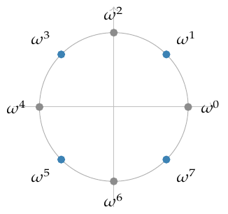
The powers $1,\omega,\dots,\omega^{n-1}$ are pairwise distinct: if $\omega^{i}=\omega^{j}$ with $0\leq i\leq j\leq n-1$ , then $\omega^{j-i}=1$ with $0\leq j-i<n$ , so primitivity (9.5, with $d=n$ ) forces $j-i=0$ . Thus $\langle\omega\rangle$ has exactly $n$ elements, all of which lie in $\mu_{n}(\mathbb{F})$ since $(\omega^{k})^{n}=(\omega^{n})^{k}=1$ . But $\lvert\mu_{n}(\mathbb{F})\rvert\leq n$ by 9.2, so the inclusion $\langle\omega\rangle\subseteq\mu_{n}(\mathbb{F})$ is an equality of $n$ -element sets. □

Over the complex numbers a primitive $n$ -th root of unity always exists, namely $\omega=e^{2\pi i/n}$ : this is the classical picture of $n$ equally spaced points on the unit circle, with the primitive roots sitting at the angles $2\pi k/n$ for $\gcd(k,n)=1$ . Over a finite field existence is more delicate, and it is exactly the finite case that matters for cryptography.

Refer to caption — Figure 1: The eight $8$ -th roots of unity in $\mathbb{C}$ , equally spaced on the unit circle at angles $2\pi k/8$ , with $\omega=e^{2\pi i/8}$ . The four primitive ones ( $k=1,3,5,7$ , exactly the $k$ coprime to $8$ ; marked in colour) each generate the whole cycle; the grey points $\omega^{0}=1$ , $\omega^{2}=i$ , $\omega^{4}=-1$ , $\omega^{6}=-i$ have orders $1,4,2,4$ and generate proper subgroups. Over a finite field the same group structure survives with the geometry stripped away—the picture to keep is the cycle, not the circle.

9.2 Existence over finite fields: the condition $n\mid q-1$

The decisive structural fact about finite fields is that their multiplicative group $\mathbb{F}_{q}^{\times}$ is cyclic of order $q-1$ (6.17); the existence theorem for roots of unity rests on it.

Theorem 9.7 (Existence and count of primitive $n$ -th roots of unity).

Let $\mathbb{F}_{q}$ be a finite field and $n\in\mathbb{N}_{>0}$ with $\gcd(n,q)=1$ (automatic when $n<p$ , where $p=\operatorname{char}\mathbb{F}_{q}$ ; equivalently, in characteristic $p$ , exactly the condition $p\nmid n$ ). Then:

1.

$\mathbb{F}_{q}$ contains a primitive $n$ -th root of unity if and only if $n\mid q-1$ .
2.

When $n\mid q-1$ , the group $\mu_{n}(\mathbb{F}_{q})$ is cyclic of order exactly $n$ , and the number of primitive $n$ -th roots of unity in $\mathbb{F}_{q}$ is $\varphi(n)$ , where $\varphi$ is Euler’s totient function (2.26).

Proof.

Let $g$ be a generator of $\mathbb{F}_{q}^{\times}$ , which is cyclic of order $q-1$ by 6.17.

( $\Rightarrow$ ) Suppose $\omega$ is a primitive $n$ -th root of unity in $\mathbb{F}_{q}$ . Then $\omega\in\mathbb{F}_{q}^{\times}$ has order $n$ by 9.3, and by Lagrange’s theorem the order of an element divides the group order $q-1$ (Corollary 3.30). Hence $n\mid q-1$ .

( $\Leftarrow$ ) Suppose $n\mid q-1$ , say $q-1=nm$ . Set $\omega=g^{m}$ . Then $\omega^{n}=g^{mn}=g^{q-1}=1$ , so $\omega\in\mu_{n}(\mathbb{F}_{q})$ . Its order is

\operatorname{ord}(\omega)=\operatorname{ord}(g^{m})=\frac{\operatorname{ord}(% g)}{\gcd(m,\operatorname{ord}(g))}=\frac{q-1}{\gcd(m,q-1)}=\frac{q-1}{m}=n,

using the order-of-a-power formula (Corollary 3.23) together with $m\mid q-1$ (so $\gcd(m,q-1)=m$ ). Thus $\omega$ is a primitive $n$ -th root of unity, and by 9.6, $\mu_{n}(\mathbb{F}_{q})=\langle\omega\rangle$ is cyclic of order exactly $n$ .

Count. In the cyclic group $\mu_{n}(\mathbb{F}_{q})=\langle\omega\rangle$ of order $n$ , the element $\omega^{k}$ has order $n/\gcd(k,n)$ , again by Corollary 3.23. This equals $n$ precisely when $\gcd(k,n)=1$ , and the number of $k\in\{0,1,\dots,n-1\}$ with $\gcd(k,n)=1$ is by definition $\varphi(n)$ (2.26). Hence there are exactly $\varphi(n)$ primitive $n$ -th roots of unity.

(A side note on the coprimality hypothesis. The condition $\gcd(n,q)=1$ is what guarantees that $X^{n}-1$ is separable— $\gcd(X^{n}-1,nX^{n-1})=1$ when $n\neq 0$ in $\mathbb{F}_{q}$ —hence has $n$ distinct roots in a splitting field over $\mathbb{F}_{q}$ (5.40); that all $n$ of them lie in $\mathbb{F}_{q}$ itself is exactly the condition $n\mid q-1$ . If $p=\operatorname{char}\mathbb{F}_{q}$ divided $n$ , then $X^{n}-1$ would have repeated roots and $\mu_{n}(\mathbb{F}_{q})$ would be strictly smaller. But $n\mid q-1$ already forces $\gcd(n,q)=1$ , since $\gcd(q-1,q)=1$ , so the hypothesis is in fact subsumed.) □

Remark 9.8.

The proof shows that for a finite field the clean statement is simply: $\mathbb{F}_{q}$ has a primitive $n$ -th root of unity $\iff n\mid q-1$ , with no separate coprimality side-condition, because $n\mid q-1$ automatically makes $n$ coprime to $q$ . We stated the condition $\gcd(n,q)=1$ explicitly only to flag the role of the characteristic.

Example 9.9.

Take $\mathbb{F}_{q}=\mathbb{F}_{p}$ with $p=7$ . Here $q-1=6$ , and $3$ is a generator of $\mathbb{F}_{7}^{\times}$ : its successive powers are $3,2,6,4,5,1$ , all six nonzero residues (Example 6.21). For $n=3\mid 6$ , set $m=6/3=2$ and $\omega=3^{2}=2$ . Indeed $2^{1}=2$ , $2^{2}=4$ , $2^{3}=8\equiv 1$ , so $\omega=2$ has order $3$ and $\mu_{3}(\mathbb{F}_{7})=\{1,2,4\}$ . There are $\varphi(3)=2$ primitive cube roots of unity, namely $2$ and $4$ . By contrast $4\nmid 6$ , so $\mathbb{F}_{7}$ has no primitive $4$ -th root of unity: $X^{4}-1=(X^{2}-1)(X^{2}+1)$ , and $X^{2}+1$ is irreducible over $\mathbb{F}_{7}$ because it has no root there, $-1$ not being a square modulo $7$ .

Remark 9.10 (Two-adicity and FFT-friendly primes).

For the fast algorithms below it is desirable that $n$ be a power of two, or at least smooth—a product of small primes, ideally with many factors of two. 9.7 shows this is possible exactly when $2^{k}\mid q-1$ . The largest $k$ with $2^{k}\mid q-1$ is called the two-adicity of the field. Designers deliberately choose primes $p$ with high two-adicity—so that $p-1=2^{k}\cdot c$ for large $k$ —as scalar fields in proof systems precisely so that large smooth evaluation domains exist. Both Pasta primes—those underlying the Pallas and Vesta curves of 10—satisfy $2^{32}\mid p-1$ , with two-adicity exactly $32$ (the primes are specified in §5.4.9.6, “Pallas and Vesta”, of the Zcash protocol specification), so each Pasta field contains primitive $2^{k}$ -th roots of unity for every $k\leq 32$ , furnishing power-of-two evaluation domains of every size up to $2^{32}$ ; this is what makes the entire machinery of this section available to Halo 2 and Orchard.

9.3 The evaluation domain $H$ and its vanishing polynomial

We now fix the central object of this section.

Definition 9.11 (Evaluation domain).

Let $\mathbb{F}$ be a field containing a primitive $n$ -th root of unity $\omega$ . The evaluation domain of order $n$ is the multiplicative subgroup

H=\langle\omega\rangle=\{\,1,\omega,\omega^{2},\dots,\omega^{n-1}\,\}=\mu_{n}(% \mathbb{F})\subseteq\mathbb{F}^{\times},

a cyclic group of order $n$ by 9.6. We index its elements as $\omega^{0},\omega^{1},\dots,\omega^{n-1}$ , and abbreviate $\omega^{i}$ by $h_{i}$ when convenient. Both $\mathbb{F}$ and $\omega$ remain fixed for the rest of the section.

Because $H$ is a multiplicative group, it is closed under products and inverses, and $1\in H$ . These elementary facts are exactly what make $H$ substantially more useful than an arbitrary set of $n$ interpolation points: cosets, products, and shifts of $H$ interact algebraically. The single most important polynomial attached to $H$ is the one that vanishes precisely on it.

Definition 9.12 (Vanishing polynomial).

The vanishing polynomial (or zerofier) of $H$ is

Z_{H}(X)=\prod_{h\in H}(X-h)\in\mathbb{F}[X].

On a generic $n$ -point set the vanishing polynomial (5.33) is an unstructured product of $n$ linear factors. On the group $H$ it collapses.

Theorem 9.13 (Closed form and factorisation of the vanishing polynomial).

With $H=\mu_{n}(\mathbb{F})$ of order $n$ generated by a primitive $n$ -th root of unity $\omega$ ,

Z_{H}(X)\;=\;X^{n}-1\;=\;\prod_{i=0}^{n-1}\bigl{(}X-\omega^{i}\bigr{)}.

Moreover $Z_{H}$ is separable: it has $n$ distinct roots and $\gcd(Z_{H},Z_{H}^{\prime})=1$ .

Proof.

Every $h\in H$ satisfies $h^{n}=1$ , hence is a root of $X^{n}-1$ . The $n$ elements of $H$ are distinct (9.6), so $X^{n}-1$ has $n$ distinct roots, namely all of $H$ , and factors as $X^{n}-1=c\prod_{h\in H}(X-h)$ for some constant $c\in\mathbb{F}^{\times}$ by iterating the factor theorem (5.36, with the degree leaving no room for further factors). Comparing leading coefficients—both $X^{n}-1$ and the product are monic—gives $c=1$ , whence $X^{n}-1=\prod_{h\in H}(X-h)=Z_{H}(X)$ .

For separability, the formal derivative is $Z_{H}^{\prime}(X)=nX^{n-1}$ (5.37). The existence of the $n$ distinct roots already forces $\operatorname{char}\mathbb{F}\nmid n$ : if $\operatorname{char}\mathbb{F}=\ell$ divided $n$ , say $n=\ell m$ , the freshman’s dream (6.13) would give $X^{n}-1=(X^{m}-1)^{\ell}$ , a polynomial with at most $m<n$ distinct roots—a contradiction. Hence $n\neq 0$ in $\mathbb{F}$ , so $nX^{n-1}$ is nonzero at every element of $H$ , since each is nonzero. Thus it has no root in common with $X^{n}-1$ , so $\gcd(Z_{H},Z_{H}^{\prime})=1$ and $Z_{H}$ is separable (5.40). □

The contraposition through the freshman’s dream is worth isolating as a device: it converts a root count ( $n$ distinct $n$ -th roots of unity exist) into a characteristic condition ( $\operatorname{char}\mathbb{F}\nmid n$ ), and thereby licenses dividing by $n$ in $\mathbb{F}$ —which the closed forms below do constantly.

The closed form $Z_{H}(X)=X^{n}-1$ is the workhorse of polynomial proof systems: testing whether a polynomial $f$ vanishes on all of $H$ reduces to checking divisibility by $X^{n}-1$ , which one can verify by exhibiting a quotient $t(X)$ with $f(X)=t(X)(X^{n}-1)$ . Moreover, evaluating $Z_{H}$ at any point costs a single exponentiation $X^{n}$ , not $n$ multiplications. We record two structural consequences.

Proposition 9.14 (Cosets and shifts).

Let $\gamma\in\mathbb{F}^{\times}$ and let $\gamma H=\{\gamma h:h\in H\}$ be the corresponding coset (3.27). Then the polynomial vanishing on $\gamma H$ is

Z_{\gamma H}(X)=\prod_{h\in H}(X-\gamma h)=X^{n}-\gamma^{n}.

In particular, distinct cosets of $H$ in $\mathbb{F}^{\times}$ have vanishing polynomials $X^{n}-c$ for distinct constants $c=\gamma^{n}$ , and the cosets of $H$ partition $\mathbb{F}^{\times}$ (3.28) into translates of $H$ , on each of which $X^{n}$ is constant.

Proof.

Substitute $Y=X/\gamma$ :

\prod_{h\in H}(X-\gamma h)=\gamma^{n}\prod_{h\in H}(Y-h)=\gamma^{n}(Y^{n}-1)=% \gamma^{n}\bigl{(}(X/\gamma)^{n}-1\bigr{)}=X^{n}-\gamma^{n},

using 9.13 for the middle equality. The constant is $c=\gamma^{n}$ , and

\gamma_{1}H=\gamma_{2}H\iff\gamma_{1}/\gamma_{2}\in H\iff(\gamma_{1}/\gamma_{2% })^{n}=1\iff\gamma_{1}^{n}=\gamma_{2}^{n},

so distinct cosets give distinct constants $c$ . □

Lemma 9.15 (Finite geometric series).

Let $\mathbb{F}$ be a field, $\zeta\in\mathbb{F}$ with $\zeta\neq 1$ , and $n\geq 1$ . Then

\sum_{i=0}^{n-1}\zeta^{i}=\frac{\zeta^{n}-1}{\zeta-1}.

Proof.

Write $S=1+\zeta+\zeta^{2}+\cdots+\zeta^{n-1}$ . Multiplying by $\zeta$ advances every term one slot:

\zeta S=\zeta+\zeta^{2}+\cdots+\zeta^{n-1}+\zeta^{n}.

In the difference $\zeta S-S$ , the terms $\zeta,\zeta^{2},\dots,\zeta^{n-1}$ appear in both lines and cancel; only the two extremes survive:

(\zeta-1)\,S\;=\;\zeta S-S\;=\;\zeta^{n}-1.

Since $\zeta\neq 1$ , the factor $\zeta-1$ is invertible, and dividing by it yields the claim. □

Proposition 9.16 (Sum of roots of unity).

If $n>1$ then $\sum_{i=0}^{n-1}\omega^{i}=0$ , and more generally for any integer $k$ ,

\sum_{i=0}^{n-1}\omega^{ki}=\begin{cases}n&\text{if }n\mid k,\\[2.0pt] 0&\text{if }n\nmid k.\end{cases}

Proof.

If $n\mid k$ , then $\omega^{ki}=(\omega^{n})^{ki/n}=1$ for each $i$ , so the sum is $n$ . If $n\nmid k$ , set $\zeta=\omega^{k}\neq 1$ (since $\omega$ has order $n$ , we have $\omega^{k}=1\iff n\mid k$ by 9.5), and 9.15 gives

\sum_{i=0}^{n-1}\zeta^{i}=\frac{\zeta^{n}-1}{\zeta-1}=\frac{(\omega^{n})^{k}-1% }{\zeta-1}=\frac{1-1}{\zeta-1}=0,

the denominator being nonzero because $\zeta\neq 1$ . The first claim is the case $k=1$ , valid for $n>1$ since then $n\nmid 1$ . □

Remark 9.17 (Rotation makes the vanishing inevitable).

For $n\nmid k$ there is also a proof with no formula at all. The $n$ terms of $\sum_{i}\omega^{ki}$ run through the subgroup $\langle\zeta\rangle$ generated by $\zeta=\omega^{k}$ , each element appearing equally often; multiplying the sum by $\zeta$ merely rotates that cycle one notch—each term advances to the next, the last wrapping around to the first—so the sum satisfies $\zeta S=S$ . A quantity invariant under scaling by something other than $1$ can only be zero: $(\zeta-1)S=0$ with $\zeta\neq 1$ forces $S=0$ . The balanced cycle of 1 is this argument made visible.

Remark 9.18 (Why “orthogonality”).

Call two vectors in $\mathbb{F}^{n}$ orthogonal when their standard inner product (8.21) vanishes. For each frequency $k$ let $v_{k}=(1,\omega^{k},\omega^{2k},\dots,\omega^{(n-1)k})$ be its vector of powers, and let $\bar{v}_{k}=(1,\omega^{-k},\omega^{-2k},\dots,\omega^{-(n-1)k})$ be the same construction run with $\omega^{-1}$ in place of $\omega$ : the mirror of $v_{k}$ , walking the cycle in the opposite direction, in the role the complex conjugate plays classically (on the unit circle $\bar{z}=z^{-1}$ ). Then $\langle\bar{v}_{k},\,v_{k^{\prime}}\rangle=\sum_{i}\omega^{i(k^{\prime}-k)}$ , which 9.16 evaluates to $0$ for $k\neq k^{\prime}$ and to $n$ for $k=k^{\prime}$ : distinct frequency vectors are orthogonal, and each pairs with its own mirror to $n$ . (Which factor carries the mirror is a convention: with the roles exchanged the exponent is $k-k^{\prime}$ , and the criterion $n\mid k^{\prime}-k$ is symmetric, so the verdict is the same; the order here matches the product $\overline{V}\,V$ computed in 9.29.) This is the finite-field counterpart of the orthogonality of the exponentials $\theta\mapsto e^{2\pi ik\theta}$ in classical Fourier analysis, the balanced trip around the cycle replacing the integral over the circle. It is the engine of the inverse-transform proof below (9.29): there the $v_{k}$ appear as the columns of the transform matrix, so in the inverse sum every wrong frequency’s contribution rides on one of these vanishing pairings and cancels, while the right one survives $n$ -fold and the $1/n$ rescales it.

9.4 The Lagrange basis on $H$

Attention now passes from the group $H$ to the polynomials we study on it. Since $H$ has exactly $n$ points, values on $H$ pin down polynomials of degree less than $n$ (5.20); the basis adapted to this situation is the Lagrange basis of §5.7, which on the group $H$ acquires a closed form it has on no generic point set.

Definition 9.19.

Let $\mathbb{F}[X]_{<n}$ denote the $\mathbb{F}$ -vector space of polynomials of degree strictly less than $n$ , together with the zero polynomial. It has the monomial basis $\{1,X,\dots,X^{n-1}\}$ (8.14), so $\dim_{\mathbb{F}}\mathbb{F}[X]_{<n}=n$ (8.17).

Definition 9.20.

For each $i\in\{0,1,\dots,n-1\}$ , the $i$ -th Lagrange basis polynomial for $H=\{\omega^{0},\dots,\omega^{n-1}\}$ is

L_{i}(X)\;=\;\prod_{\begin{subarray}{c}j=0\\ j\neq i\end{subarray}}^{n-1}\frac{X-\omega^{j}}{\omega^{i}-\omega^{j}}\;\in\;% \mathbb{F}[X]_{<n},

the basis polynomial $\ell_{i}$ of 5.30 for the nodes $\omega^{0},\dots,\omega^{n-1}$ .

Proposition 9.21 (Interpolation property).

The polynomials $L_{0},\dots,L_{n-1}$ satisfy the Kronecker-delta conditions

L_{i}(\omega^{j})=\delta_{ij}=\begin{cases}1&i=j,\\ 0&i\neq j,\end{cases}

they form a basis of $\mathbb{F}[X]_{<n}$ , and they give the unique interpolant: for any data $(v_{0},\dots,v_{n-1})\in\mathbb{F}^{n}$ , the polynomial

f(X)=\sum_{i=0}^{n-1}v_{i}\,L_{i}(X)

is the unique element of $\mathbb{F}[X]_{<n}$ with $f(\omega^{i})=v_{i}$ for all $i$ .

Proof.

Each $L_{i}$ is well defined and of degree $n-1$ because the nodes $\omega^{j}$ are distinct (9.6), so the denominators $\omega^{i}-\omega^{j}$ with $j\neq i$ are nonzero. The delta conditions, the interpolation $f(\omega^{j})=v_{j}$ , and the uniqueness are 5.30 (with (4)) applied to these nodes with $d=n-1$ ; uniqueness rests, as there, on the root count: two interpolants in $\mathbb{F}[X]_{<n}$ differ by a polynomial of degree $<n$ with $n$ distinct roots, which is the zero polynomial (5.18). It remains to see that the $L_{i}$ form a basis of $\mathbb{F}[X]_{<n}$ . They are linearly independent: if $\sum_{i}c_{i}L_{i}=0$ , evaluation at $\omega^{j}$ yields $c_{j}=0$ for every $j$ (8.11). Being $n$ independent vectors in the $n$ -dimensional space $\mathbb{F}[X]_{<n}$ (9.19), they form a basis (8.17). □

The root-count step deserves a name, for it recurs: to prove two polynomials of degree $<n$ equal, show they agree on all $n$ points of $H$ . We use this root-count device for the uniqueness above, for 9.24, and for Example 9.25 below.

On a generic point set the Lagrange polynomials admit no closed form simpler than the defining product. On the group $H$ they collapse to a compact expression involving the vanishing polynomial.

Theorem 9.22 (Closed form of the Lagrange basis on $H$ ).

For $H=\mu_{n}(\mathbb{F})$ with primitive root $\omega$ , and for each $i$ ,

L_{i}(X)\;=\;\frac{\omega^{i}}{n}\cdot\frac{X^{n}-1}{X-\omega^{i}}\;=\;\frac{% \omega^{i}\,(X^{n}-1)}{n\,(X-\omega^{i})}.

In particular, dividing out one linear factor and scaling yields all $n$ Lagrange polynomials from the single polynomial $Z_{H}(X)=X^{n}-1$ .

Proof.

Fix $i$ . From 9.13, $Z_{H}(X)=\prod_{j=0}^{n-1}(X-\omega^{j})$ , so

\frac{Z_{H}(X)}{X-\omega^{i}}=\prod_{\begin{subarray}{c}j=0\\ j\neq i\end{subarray}}^{n-1}(X-\omega^{j}),

which is exactly the numerator of $L_{i}$ in 9.20. It remains to evaluate the denominator $\prod_{j\neq i}(\omega^{i}-\omega^{j})$ . Writing $Z_{H}=(X-\omega^{i})\,g$ with $g=\prod_{j\neq i}(X-\omega^{j})$ , the product rule (5.38) gives $Z_{H}^{\prime}=g+(X-\omega^{i})\,g^{\prime}$ , so

Z_{H}^{\prime}(\omega^{i})=g(\omega^{i})=\prod_{\begin{subarray}{c}j=0\\ j\neq i\end{subarray}}^{n-1}(\omega^{i}-\omega^{j})

—the derivative at a simple root equals the product of the differences to the other roots, the computation already made for simple roots in the proof of 5.40. Concretely $Z_{H}^{\prime}(X)=nX^{n-1}$ , so

Z_{H}^{\prime}(\omega^{i})=n\,(\omega^{i})^{n-1}=n\,\omega^{in}\,\omega^{-i}=n% \cdot 1\cdot\omega^{-i}=\frac{n}{\omega^{i}},

using $\omega^{in}=(\omega^{n})^{i}=1$ . Therefore

L_{i}(X)=\frac{Z_{H}(X)/(X-\omega^{i})}{Z_{H}^{\prime}(\omega^{i})}=\frac{(X^{% n}-1)/(X-\omega^{i})}{n/\omega^{i}}=\frac{\omega^{i}\,(X^{n}-1)}{n\,(X-\omega^% {i})},

as claimed. □

Remark 9.23 (Barycentric form).

The closed form renders the barycentric interpolation formula on $H$ especially clean. Writing $f(X)=\sum_{i}v_{i}L_{i}(X)$ and substituting 9.22,

f(X)=\frac{X^{n}-1}{n}\sum_{i=0}^{n-1}\frac{\omega^{i}\,v_{i}}{X-\omega^{i}}.

Evaluating $f$ at a point $z\notin H$ thus costs one evaluation of $z^{n}-1$ and $n$ terms of the sum, with no per-point polynomial reconstruction. A verifier can use this formula when the values $v_{i}$ are known, as for public-input polynomials; a commitment to hidden values does not by itself permit this evaluation.

Proposition 9.24 (Lagrange polynomials sum to one).

The Lagrange basis polynomials for $H$ satisfy $\sum_{i=0}^{n-1}L_{i}(X)=1$ identically.

Proof.

The polynomial $g(X)=\sum_{i}L_{i}(X)-1$ lies in $\mathbb{F}[X]_{<n}$ and vanishes at every $\omega^{j}$ , because $\sum_{i}L_{i}(\omega^{j})=\sum_{i}\delta_{ij}=1$ (9.21). By the root-count device—a polynomial of degree $<n$ with $n$ distinct roots is zero (5.18)— $g\equiv 0$ . □

Example 9.25 (The all-ones value vector).

The constant polynomial $1$ interpolates the data $v_{i}=1$ for all $i$ ; 9.24 is the statement $\sum_{i}1\cdot L_{i}=1$ . Likewise the values of $X$ on $H$ are $v_{i}=\omega^{i}$ , and, for $n\geq 2$ , 9.21 gives $\sum_{i}\omega^{i}L_{i}(X)=X$ : both sides have degree $<n$ and agree on all of $H$ , so the root-count device applies. We invoke these identities constantly when rewriting monomials in the Lagrange basis.

9.5 Evaluation and interpolation as mutually inverse linear maps

An element of $\mathbb{F}[X]_{<n}$ admits two natural descriptions: by its $n$ coefficients, or by its $n$ values on $H$ . Both are coordinate systems on the same $n$ -dimensional vector space, and passage between them is a linear isomorphism—the specialisation to $H$ of the evaluation isomorphism met for general nodes in 5.32.

Definition 9.26 (Evaluation map).

The evaluation map on $H$ is the $\mathbb{F}$ -linear map (8.18)

\mathrm{ev}_{H}\colon\mathbb{F}[X]_{<n}\longrightarrow\mathbb{F}^{n},\qquad% \mathrm{ev}_{H}(f)=\bigl{(}f(\omega^{0}),f(\omega^{1}),\dots,f(\omega^{n-1})% \bigr{)}.

Linearity is immediate from $(af+bg)(\omega^{i})=af(\omega^{i})+bg(\omega^{i})$ , an instance of 5.16.

Theorem 9.27 (Evaluation and interpolation are mutually inverse).

The evaluation map $\mathrm{ev}_{H}$ is a vector-space isomorphism. Its inverse is the interpolation map

\mathrm{int}_{H}\colon\mathbb{F}^{n}\longrightarrow\mathbb{F}[X]_{<n},\qquad% \mathrm{int}_{H}(v_{0},\dots,v_{n-1})=\sum_{i=0}^{n-1}v_{i}\,L_{i}(X).

That is, $\mathrm{int}_{H}\circ\mathrm{ev}_{H}=\operatorname{id}_{\mathbb{F}[X]_{<n}}$ and $\mathrm{ev}_{H}\circ\mathrm{int}_{H}=\operatorname{id}_{\mathbb{F}^{n}}$ .

Proof.

Both maps are linear and act between spaces of the same finite dimension $n$ , so verifying one composition would suffice (a one-sided inverse makes $\mathrm{ev}_{H}$ injective, hence surjective by rank–nullity, 8.19); we check both for clarity. For $v\in\mathbb{F}^{n}$ , the polynomial $\mathrm{int}_{H}(v)=\sum_{i}v_{i}L_{i}$ has value $\sum_{i}v_{i}L_{i}(\omega^{j})=v_{j}$ at $\omega^{j}$ by 9.21, so $\mathrm{ev}_{H}(\mathrm{int}_{H}(v))=v$ . For $f\in\mathbb{F}[X]_{<n}$ , the polynomial $\mathrm{int}_{H}(\mathrm{ev}_{H}(f))=\sum_{i}f(\omega^{i})L_{i}$ is, by the uniqueness clause of 9.21, the unique degree- $<n$ polynomial taking the values $f(\omega^{i})$ on $H$ —which is $f$ itself. Hence the two maps are inverse; in particular $\mathrm{ev}_{H}$ is bijective and linear, i.e. an isomorphism (8.18). □

In coordinates, $\mathrm{ev}_{H}$ is given by a matrix, which we name here because it is the bridge to the Fourier transform. The notation is worth fixing once, since §8 did not need it: an $n\times n$ matrix over $\mathbb{F}$ is a doubly indexed family $A=(A_{ik})_{0\leq i,k\leq n-1}$ of elements of $\mathbb{F}$ , acting on a vector $c\in\mathbb{F}^{n}$ by $(Ac)_{i}=\sum_{k}A_{ik}c_{k}$ —the general form, written out through the standard basis (Example 8.15), of a linear map $\mathbb{F}^{n}\to\mathbb{F}^{n}$ . The product of two matrices is defined so that $(AB)\,c=A(Bc)$ , which forces $(AB)_{ij}=\sum_{k}A_{ik}B_{kj}$ ; the identity matrix $I$ , with entries $\delta_{ik}$ , acts as the identity map; and $A$ is invertible if some matrix $A^{-1}$ satisfies $A^{-1}A=AA^{-1}=I$ .

Definition 9.28 (Vandermonde / DFT matrix).

Let $f(X)=\sum_{k=0}^{n-1}c_{k}X^{k}$ have coefficient vector $c=(c_{0},\dots,c_{n-1})$ . Then $\mathrm{ev}_{H}(f)$ has $i$ -th entry $f(\omega^{i})=\sum_{k}c_{k}\,\omega^{ik}$ . Thus, relative to the monomial basis on $\mathbb{F}[X]_{<n}$ and the standard basis on $\mathbb{F}^{n}$ , the Vandermonde matrix

V=\bigl{(}\omega^{ik}\bigr{)}_{0\leq i,k\leq n-1}=\begin{pmatrix}1&1&1&\cdots&% 1\\ 1&\omega&\omega^{2}&\cdots&\omega^{n-1}\\ 1&\omega^{2}&\omega^{4}&\cdots&\omega^{2(n-1)}\\ \vdots&&&&\vdots\\ 1&\omega^{n-1}&\omega^{2(n-1)}&\cdots&\omega^{(n-1)^{2}}\end{pmatrix}

—rows indexed by the evaluation point $\omega^{i}$ , columns by the power $k$ —represents $\mathrm{ev}_{H}$ , so that $\mathrm{ev}_{H}(f)=Vc$ . We call $V$ the (discrete Fourier) transform matrix on $H$ .

Theorem 9.29 (Invertibility and the inverse transform).

The matrix $V$ of 9.28 is invertible, with

(V^{-1})_{k,i}=\frac{1}{n}\,\omega^{-ik}.

Equivalently, $V^{-1}=\tfrac{1}{n}\overline{V}$ , where $\overline{V}=(\omega^{-ik})_{i,k}$ is the transform matrix built from $\omega^{-1}$ (itself a primitive $n$ -th root of unity). Consequently the coefficient and value representations are related by the mutually inverse formulas

c_{k}=\frac{1}{n}\sum_{i=0}^{n-1}f(\omega^{i})\,\omega^{-ik},\qquad f(\omega^{% i})=\sum_{k=0}^{n-1}c_{k}\,\omega^{ik}.

Proof.

First note that $\omega^{-1}=\omega^{n-1}$ has order $n$ by Corollary 3.23 (with $\gcd(n-1,n)=1$ ), so $\overline{V}$ is again a matrix of the shape in 9.28. We show $\overline{V}V=nI$ . The $(k,k^{\prime})$ entry of $\overline{V}V$ is

\sum_{i=0}^{n-1}\omega^{-ik}\,\omega^{ik^{\prime}}=\sum_{i=0}^{n-1}\omega^{i(k% ^{\prime}-k)}.

By 9.16 this sum is $n$ if $n\mid(k^{\prime}-k)$ and $0$ otherwise; for $k,k^{\prime}\in\{0,\dots,n-1\}$ we have $n\mid(k^{\prime}-k)\iff k=k^{\prime}$ . Hence $\overline{V}V=nI$ , and the same computation with the roles of the two factors exchanged gives $V\overline{V}=nI$ . Since $n\neq 0$ in $\mathbb{F}$ (9.13), we may divide by $n$ : $V^{-1}=\tfrac{1}{n}\overline{V}$ . The component formulas write out the matrix identities $\mathrm{ev}_{H}(f)=Vc$ and $c=V^{-1}\,\mathrm{ev}_{H}(f)$ . □

Remark 9.30.

9.27 and 9.29 are two faces of one statement. The abstract face: evaluation on $H$ is an isomorphism whose inverse is Lagrange interpolation. The concrete face: that isomorphism is the matrix $V$ , and its inverse is, up to the scalar $1/n$ , the same matrix with $\omega$ replaced by $\omega^{-1}$ . The near-symmetry between a transform and its inverse—differing only by the substitution $\omega\mapsto\omega^{-1}$ and a scale $1/n$ —is the algebraic reason the fast inverse transform of 9.37 costs exactly as much as the forward one.

9.6 The number-theoretic transform and convolution

The map $\mathrm{ev}_{H}$ , read as the matrix $V$ , is the discrete Fourier transform, but over a finite field rather than over $\mathbb{C}$ . Because it involves no analytic structure—no complex exponentials, no convergence—it is called the number-theoretic transform.

Definition 9.31 (Number-theoretic transform).

Let $\omega$ be a primitive $n$ -th root of unity in $\mathbb{F}$ . The number-theoretic transform (NTT) sends the coefficient vector of a polynomial to its value vector on $H$ : it is the evaluation map $\mathrm{ev}_{H}$ written in coordinates. Explicitly, the NTT of $a=(a_{0},\dots,a_{n-1})\in\mathbb{F}^{n}$ is $\hat{a}=(\hat{a}_{0},\dots,\hat{a}_{n-1})$ with

\hat{a}_{j}=\sum_{k=0}^{n-1}a_{k}\,\omega^{jk},\qquad j=0,\dots,n-1,

each entry being the value at $\omega^{j}$ of the polynomial with coefficients $a$ . The inverse number-theoretic transform is interpolation—the recovery of the coefficients from the values—and by 9.29 it too is a single explicit sum:

a_{k}=\frac{1}{n}\sum_{j=0}^{n-1}\hat{a}_{j}\,\omega^{-jk}.

The NTT enjoys the same convolution property as the classical DFT, and this is the mechanism underlying fast polynomial multiplication. Recall that the coefficients of a product are a convolution: with $f=\sum_{i}a_{i}X^{i}$ and $g=\sum_{j}b_{j}X^{j}$ , the coefficient of $X^{k}$ in $f g$ is $\sum_{i+j=k}a_{i}b_{j}$ (5.3). The cyclic variant folds indices modulo $n$ : for $a,b\in\mathbb{F}^{n}$ , the cyclic convolution $a*b\in\mathbb{F}^{n}$ has entries

(a*b)_{k}\;=\;\sum_{\begin{subarray}{c}0\leq i,j\leq n-1\\ i+j\equiv k\pmod{n}\end{subarray}}a_{i}\,b_{j},\qquad k=0,\dots,n-1.

Theorem 9.32 (Convolution theorem).

For $f,g\in\mathbb{F}[X]_{<n}$ with $\deg f+\deg g<n$ , let $c=fg$ be their product (of degree $<n$ ). Then for every $h\in H$ ,

c(h)=f(h)\,g(h),

i.e. pointwise multiplication of value vectors corresponds to polynomial multiplication. Equivalently, writing $a,b\in\mathbb{F}^{n}$ for the coefficient vectors of $f, g$ (padded with zeros up to length $n$ ),

\widehat{a*b}_{j}=\hat{a}_{j}\,\hat{b}_{j}\qquad(j=0,\dots,n-1),

so the NTT turns convolution into entrywise multiplication.

Proof.

The first identity is the statement that evaluation at $h$ is a ring homomorphism $\mathbb{F}[X]\to\mathbb{F}$ (5.16): $(fg)(h)=f(h)\,g(h)$ . Since $\deg(fg)<n$ , interpolation recovers the product $c=fg$ from its values on the $n$ -point set $H$ (9.21), so the entrywise product of the value vectors uniquely determines $c$ .

For the convolution statement the plan is: (i) multiplication in $\mathbb{F}[X]/(X^{n}-1)$ is cyclic convolution of coefficient vectors; (ii) evaluation on $H$ is a ring isomorphism from that quotient onto $\mathbb{F}^{n}$ with entrywise operations; (iii) the degree bound rules out wrap-around, so the cyclic product is the genuine one. For (i), work in the quotient ring $\mathbb{F}[X]/(X^{n}-1)$ (4.19 and 4.20, applied to the ideal of multiples of $X^{n}-1$ , 4.17). Every class has a unique representative of degree $<n$ , by division with remainder (5.12); and multiplying two such representatives and reducing replaces each $X^{k}$ with $k\geq n$ by $X^{k-n}$ , since $X^{n}\equiv 1$ . The coefficient of $X^{k}$ in the reduced product of the representatives with coefficient vectors $a$ and $b$ is therefore $\sum_{i+j\equiv k\ (\mathrm{mod}\ n)}a_{i}b_{j}=(a*b)_{k}$ : multiplication in $\mathbb{F}[X]/(X^{n}-1)$ is cyclic convolution of coefficient vectors.

Now consider the map $[p]\mapsto\mathrm{ev}_{H}(p)$ from $\mathbb{F}[X]/(X^{n}-1)$ to $\mathbb{F}^{n}$ , where $\mathbb{F}^{n}$ is a commutative ring under entrywise addition and multiplication (the ring laws hold in each coordinate because they hold in $\mathbb{F}$ ), with multiplicative identity $(1,\dots,1)$ . The map is well defined: two representatives of a class differ by a multiple of $X^{n}-1$ , which vanishes on $H$ (9.13). It is a ring homomorphism (4.21), because evaluation at each point of $H$ is one (5.16) and the operations on $\mathbb{F}^{n}$ are entrywise. And it is bijective: classes correspond to their degree- $<n$ representatives, on which $\mathrm{ev}_{H}$ is a bijection by 9.27. Hence it is a ring isomorphism $\mathbb{F}[X]/(X^{n}-1)\xrightarrow{\ \sim\ }\mathbb{F}^{n}$ , and it sends the product of the classes of $f$ and $g$ —coefficient vector $a*b$ —to the entrywise product of $\hat{a}$ and $\hat{b}$ . This is the displayed identity. Finally, when $\deg f+\deg g<n$ , the genuine product $f g$ already has degree $<n$ , so no folding occurs, the cyclic and ordinary products coincide, and the statement computes $f g$ itself. □

Remark 9.33 (Computational significance).

9.32 reduces multiplying two degree- $<n/2$ polynomials—a quadratic-cost operation by the schoolbook method—to: transform both (NTT), multiply the value vectors entrywise ( $n$ multiplications), and transform back (inverse NTT). If the NTT runs in $O(n\log n)$ operations, the whole multiplication costs $O(n\log n)$ . The fast Fourier transform supplies that conditional.

Example 9.34 (The convolution theorem in $\mathbb{F}_{17}$ ).

In $\mathbb{F}_{17}$ , the element $\omega=4$ has $\omega^{2}=16=-1$ , so it is a primitive $4$ -th root of unity with domain $H=\{1,4,16,13\}$ . To multiply $f=1+2X$ and $g=3+X$ , pad both coefficient vectors to length $4$ and transform: $\hat{a}=(3,9,16,10)$ and $\hat{b}=(4,7,2,16)$ , the values of $f$ and of $g$ on $H$ . Multiplying entrywise gives $(12,12,15,7)$ , the values of $f g$ on $H$ , and the inverse transform returns $(3,7,2,0)$ : the coefficients of $fg=3+7X+2X^{2}$ , agreeing with the schoolbook product. At $n=4$ nothing is saved; the point is the shape of the pipeline, which becomes decisive once the transforms themselves cost $O(n\log n)$ (§9.7).

9.7 The fast Fourier transform

Computing $\hat{a}=Va$ directly from 9.28 costs $\Theta(n^{2})$ field multiplications: each of the $n$ outputs is a sum of $n$ products. The fast Fourier transform (FFT)—here a number-theoretic FFT—computes the same vector in $O(n\log n)$ operations by a divide-and-conquer recursion, provided $n$ is a power of two (or, more generally, smooth). This is where the requirement that $H$ have smooth order, 9.10, becomes indispensable.

Theorem 9.35 (Cooley–Tukey radix-2 step).

Suppose $n=2m$ and $\omega$ is a primitive $n$ -th root of unity in $\mathbb{F}$ . Given $f(X)=\sum_{k=0}^{n-1}a_{k}X^{k}$ , split its coefficients by parity into

f_{\mathrm{even}}(Y)=\sum_{k=0}^{m-1}a_{2k}\,Y^{k},\qquad f_{\mathrm{odd}}(Y)=% \sum_{k=0}^{m-1}a_{2k+1}\,Y^{k},

so that $f(X)=f_{\mathrm{even}}(X^{2})+X\,f_{\mathrm{odd}}(X^{2})$ . Then $\eta:=\omega^{2}$ is a primitive $m$ -th root of unity, and for $j=0,\dots,m-1$ ,

	$\displaystyle f(\omega^{j})$	$\displaystyle=f_{\mathrm{even}}(\eta^{j})+\omega^{j}\,f_{\mathrm{odd}}(\eta^{j% }),$		(7)
	$\displaystyle f(\omega^{j+m})$	$\displaystyle=f_{\mathrm{even}}(\eta^{j})-\omega^{j}\,f_{\mathrm{odd}}(\eta^{j% }).$		(8)

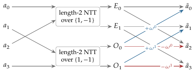
Thus the length- $n$ NTT of $a$ reduces to two length- $m$ NTTs (of the even and odd coefficient subsequences, over the domain $\langle\eta\rangle$ ) plus $O(n)$ extra operations.

Proof.

The identity $f(X)=f_{\mathrm{even}}(X^{2})+Xf_{\mathrm{odd}}(X^{2})$ regroups the sum $\sum_{k}a_{k}X^{k}$ into even-index and odd-index terms; in the odd terms one factor of $X$ is pulled out, leaving powers $X^{2k}$ . That $\eta=\omega^{2}$ is a primitive $m$ -th root of unity follows from 9.5 and the order-of-a-power formula (Corollary 3.23): $\operatorname{ord}(\omega^{2})=n/\gcd(2,n)=n/2=m$ , using $2\mid n$ .

It remains to evaluate. For (7), put $X=\omega^{j}$ ; then $X^{2}=\omega^{2j}=\eta^{j}$ , so $f(\omega^{j})=f_{\mathrm{even}}(\eta^{j})+\omega^{j}f_{\mathrm{odd}}(\eta^{j})$ . For (8), put $X=\omega^{j+m}$ ; then $X^{2}=\omega^{2j+2m}=\omega^{2j}\,\omega^{n}=\eta^{j}\cdot 1=\eta^{j}$ (since $2m=n$ and $\omega^{n}=1$ ), while the linear factor is $\omega^{j+m}=\omega^{j}\,\omega^{m}=-\omega^{j}$ . Here $\omega^{m}=-1$ , because $\omega^{m}$ has order $n/\gcd(m,n)=n/m=2$ (Corollary 3.23), and $-1$ is the unique element of order $2$ in a field: $x^{2}=1$ with $x\neq 1$ forces $(x-1)(x+1)=0$ and so $x=-1$ ; and $-1\neq 1$ , since $\operatorname{char}\mathbb{F}\nmid n$ (9.13) with $n$ even forces $\operatorname{char}\mathbb{F}\neq 2$ . Substituting, $f(\omega^{j+m})=f_{\mathrm{even}}(\eta^{j})-\omega^{j}f_{\mathrm{odd}}(\eta^{j})$ . □

The half-domain trick just used— $\omega^{m}=-1$ whenever $n=2m$ , so the second half of the outputs differs from the first only by a sign on the odd part—recurs in every radix-2 argument over an evaluation domain; it is worth remembering alongside the theorem.

Remark 9.36 (The butterfly).

Equations (7)–(8) constitute the butterfly: from the two subtransform outputs $E_{j}=f_{\mathrm{even}}(\eta^{j})$ and $O_{j}=f_{\mathrm{odd}}(\eta^{j})$ one forms the twiddle $t_{j}=\omega^{j}O_{j}$ and reads off the two outputs $E_{j}+t_{j}$ and $E_{j}-t_{j}$ . Pictorially, $E_{j}$ and $O_{j}$ sit as two nodes on the left; each is carried to both outputs on the right, the two $E_{j}$ -edges with weight $1$ and the two $O_{j}$ -edges with weights $+\omega^{j}$ and $-\omega^{j}$ ; the pair of crossing edges forms the $\times$ that names the operation. Each butterfly costs one multiplication (the twiddle) and two additions, and there are $n/2$ of them per level.

Theorem 9.37 ( $O(n\log n)$ cost of the FFT).

Let $n=2^{t}$ and let $T(n)$ be the number of field additions and multiplications the radix-2 recursion of 9.35 uses to compute a length- $n$ NTT. Then

T(n)=2\,T(n/2)+cn\quad(n>1),\qquad T(1)=O(1),

for a constant $c$ , and therefore $T(n)=O(n\log n)$ . The inverse NTT has the same cost, since it is the forward NTT with $\omega$ replaced by $\omega^{-1}$ , followed by scaling each entry by $1/n$ (9.29).

Proof.

The recursion is exactly 9.35: a length- $n$ transform calls two length- $n/2$ transforms (on the even and odd coefficient subsequences) and combines them with $n/2$ butterflies of $O(1)$ operations each, for the $c n$ overhead. Unrolling, with $n=2^{t}$ ,

T(2^{t})=2\,T(2^{t-1})+c\,2^{t}.

Divide by $2^{t}$ and set $S(t)=T(2^{t})/2^{t}$ : then $S(t)=S(t-1)+c$ , so $S(t)=S(0)+ct=O(1)+ct$ , and $T(2^{t})=2^{t}S(t)=O(2^{t})+ct\,2^{t}=O(t\,2^{t})$ . With $t=\log_{2}n$ this is $T(n)=O(n\log n)$ . (Equivalently: the recursion tree has $\log_{2}n$ levels, each performing $\Theta(n)$ total work across all subproblems at that level.) The inverse-transform claim is 9.29: the inverse is the same Cooley–Tukey recursion with $\omega^{-1}$ in place of $\omega$ (also a primitive $n$ -th root of unity), plus a final pass of $n$ divisions by $n$ , all within $O(n\log n)$ . □

Remark 9.38 (Mixed radix and smoothness).

The hypothesis that enables fast transforms is that $n$ be smooth—a product of small primes—and, crucially, that the field actually contain a primitive $n$ -th root of unity, i.e. $n\mid q-1$ (9.7). A power-of-two $n$ dividing $q-1$ is the optimal case: pure radix-2 with the cleanest butterfly.

Example 9.39 (A length- $4$ transform).

Take $n=4$ with primitive $4$ -th root $\omega$ (so $\omega^{2}=-1$ and $\omega^{4}=1$ , and $\eta=\omega^{2}=-1$ is the primitive $2$ nd root). For $f=a_{0}+a_{1}X+a_{2}X^{2}+a_{3}X^{3}$ , the two length- $2$ subtransforms over the domain $\{1,-1\}$ —each itself a single butterfly, with twiddle $\eta^{0}=1$ —are

E=(a_{0}+a_{2},\;a_{0}-a_{2}),\qquad O=(a_{1}+a_{3},\;a_{1}-a_{3}),

and the butterflies give

\hat{a}_{0}=E_{0}+\omega^{0}O_{0},\quad\hat{a}_{2}=E_{0}-\omega^{0}O_{0},\quad% \hat{a}_{1}=E_{1}+\omega^{1}O_{1},\quad\hat{a}_{3}=E_{1}-\omega^{1}O_{1}.

(Note the output indexing: outputs $j$ and $j+m$ pair up, per (7)–(8).) This uses $2$ subtransforms of $2$ additions each plus $2$ butterflies of $2$ additions each ( $n/2=2$ per level, 9.36)—together $2$ twiddle multiplications and $8$ additions—versus $16$ coefficient-products and $12$ additions for the direct $4\times 4$ matrix multiply; and the gap widens as $n$ grows.

9.8 The role of smooth multiplicative domains in polynomial proof systems

This section closes by assembling the pieces into the reason these domains form the substrate of Halo 2 and Orchard. A proof system of the polynomial type encodes a computation as a system of polynomial identities and convinces a verifier that those identities hold. The evaluation domain $H=\mu_{n}$ is where the encoding lives—the $n$ -step table of the section’s opening is laid out on the $n$ points of $H$ —and every property proved above is load-bearing.

Remark 9.40 (The roles played by $H$ , $Z_{H}$ , the Lagrange basis, and the FFT).

•

Witnesses as evaluations on $H$ . A prover lays out the trace of a computation as the values of one or more polynomials on the $n$ points of $H$ . By 9.27 this is the same data as a polynomial of degree $<n$ ; the prover may move freely between the value (Lagrange) representation, natural for stating constraints row by row, and the coefficient representation, natural for committing and for low-degree testing. The change of representation is the (inverse) NTT.
•

Constraints as divisibility by $Z_{H}$ . “Constraint polynomial $C$ holds on every row” means $C$ vanishes on all of $H$ , which by 9.13 means exactly that $Z_{H}=X^{n}-1$ divides $C$ . The prover demonstrates this by exhibiting a quotient $t$ with $C(X)=t(X)\,(X^{n}-1)$ . The inexpensive closed form $Z_{H}(X)=X^{n}-1$ —one exponentiation to evaluate—is what makes this check cheap at a random point. 9.14 extends the same technique to cosets $\gamma H$ , used to separate quotient and remainder domains.
•

Lagrange selectors. The Lagrange polynomials $L_{i}$ of 9.20 are selectors: $L_{i}$ is $1$ on row $i$ and $0$ elsewhere (9.21), so boundary and instance constraints (e.g. “the first row equals the public input”) become $L_{0}\cdot(\dots)$ . The closed form and the barycentric formula (9.22, 9.23) let the verifier evaluate these at a random challenge in $O(n)$ or even $O(\log n)$ field operations rather than reconstructing polynomials.
•

Group structure for permutations and shifts. Because $H$ is a cyclic group (9.11), multiplication by $\omega$ is the cyclic “next-row” shift $\omega^{i}\mapsto\omega^{i+1}$ . Constraints relating a row to its neighbour become $f(\omega X)$ versus $f(X)$ ; permutation arguments—the heart of Halo 2’s copy constraints—rest on the action of the group on itself and on its cosets. An arbitrary set of $n$ points offers none of this.
•

Smoothness for speed. Provers manipulate polynomials of size $n$ (often after blowing the domain up by a small constant factor for low-degree testing). Every transform between representations, every multiplication, every coset evaluation is an NTT. By 9.37 these cost $O(n\log n)$ instead of $O(n^{2})$ —the difference between feasible and infeasible at the sizes used in practice—provided $n$ is smooth and $\mathbb{F}_{q}$ contains a primitive $n$ -th root of unity. By 9.7 that requires $n\mid q-1$ ; by 9.10 this is why high-two-adicity primes are chosen for the scalar fields of the Pallas and Vesta curves (10).

In summary: the existence condition $n\mid q-1$ (9.7) supplies the group $H$ ; the group supplies the clean vanishing polynomial (9.13), the closed-form Lagrange basis (9.22), and the evaluation/interpolation isomorphism (9.27); and smoothness of $n$ supplies the $O(n\log n)$ FFT (9.37). Together these discharge both demands of the section’s opening—a structured point set on which an execution trace can live, and $O(n\log n)$ multiplication and interpolation on it—and they are exactly the ingredients a polynomial proof system requires, which is why such systems rest on smooth multiplicative evaluation domains and on the fields that contain them.