The Zcash ArboretumI–IX The Complete Arboretum
Contents
PDF
Theme

5 Polynomials over a field

Throughout this section F denotes a field. The section constructs the ring F[X] with its division, gcd and factorisation theory, and proves that a nonzero polynomial of degree d over a field has at most d roots. From this bound it derives Lagrange interpolation (§5.7) and the Schwartz–Zippel lemma (§5.10), which justifies the polynomial identity testing of the later volumes: two polynomials encoding a computation are compared by evaluating both at one random α, not coefficient by coefficient at the cost of reading the computation. Halo 2 and Zcash Orchard use these results in their polynomial commitment schemes and their arithmetisation, the encoding of a computation as identities between polynomials; polynomials also underlie finite fields and error-correcting codes.

5.1 The polynomial ring

A polynomial is a formal expression, a finite list of coefficients, and not a function: evaluating it yields a function, which over a finite field carries less information than the polynomial (§5.9).

Definition 5.1 (Polynomial).

A polynomial over F in the indeterminate X is a formal expression

f=a0+a1⁢X+a2⁢X2+⋯+an⁢Xn=∑i=0nai⁢Xi,

where n∈ℕ={0,1,2,…} and the coefficients a0,…,an lie in F. Formally, f is identified with its coefficient sequence (a0,a1,a2,…), in which only finitely many entries are nonzero. Two polynomials are equal precisely when their coefficient sequences agree term by term:

∑iai⁢Xi=∑ibi⁢Xi⟺ai=bi⁢ for every ⁢i∈ℕ.

The symbol X is an indeterminate (a formal variable): it is not an element of F and denotes no particular value; it is a placeholder organising the coefficients. The set of all polynomials over F in X is denoted F[X].

Remark 5.2 (The sequence model).

In the rigorous form of 5.1, F[X] is the set of all functions a:ℕ→F that are eventually zero: there is some N with a(i)=0 for all i>N. The expression ∑iaiXi is notation for the sequence (a0,a1,…), and the two viewpoints are used interchangeably: the arithmetic of sequences defined next is the arithmetic the notation suggests.

Definition 5.3 (Ring operations on F[X]).

Let f=∑iaiXi and g=∑ibiXi lie in F[X], with the shorter coefficient sequence zero-padded so that both run over the same index set. Their sum and product are

f+g=∑i≥0(ai+bi)⁢Xi,f⁢g=∑k≥0ck⁢Xkwhereck=∑i+j=kai⁢bj=∑i=0kai⁢bk−i.

The coefficient ck is the convolution of the two coefficient sequences. Both defining sums are finite—only finitely many ai and bj are nonzero, hence only finitely many ck are nonzero—so the sum and the product are again polynomials.

The convolution formula results from multiplying out the product (∑iaiXi)(∑jbjXj) and collecting like powers of X using Xi⋅Xj=Xi+j; as a convolution it involves no substitution of a value for X. The proof of the ring axioms (4.1) likewise involves no evaluation: it writes the coefficient of Xm on each side of an identity as a finite sum over index decompositions, then reindexes or regroups that sum, as in the associativity step below.

Theorem 5.4 (F[X] is a commutative ring).

With the operations of 5.3, the set F[X] is a commutative ring whose additive identity is the zero polynomial 0=(0,0,0,…) and whose multiplicative identity is the constant polynomial 1=(1,0,0,…). Moreover the map c↦(c,0,0,…) embeds F into F[X] as a subring, the constant polynomials; in this sense F⊆F[X].

Proof.

Additive structure. Addition is coordinatewise, so its commutativity and associativity are inherited directly from the corresponding laws of the additive group of F, the sequence (0,0,…) is an additive identity, and (−a0,−a1,…) is an additive inverse of (a0,a1,…). Hence (F[X],+) is an abelian group.

Commutativity of multiplication. The coefficient of Xk in fg is ∑i+j=kaibj; reindexing the sum by (i,j)↦(j,i) and using commutativity of multiplication in F,

∑i+j=kai⁢bj=∑i+j=kbi⁢aj,

which is the coefficient of Xk in gf.

Associativity of multiplication. Write h=∑lclXl. The coefficient of Xm in (fg)h is

∑k+l=m(∑i+j=kai⁢bj)⁢cl=∑i+j+l=mai⁢bj⁢cl,

and expanding f(gh) instead produces ∑i+j+l=mai(bjcl), the same symmetric triple sum by associativity in F. Hence (fg)h=f(gh) coefficient by coefficient.

Distributivity. The coefficient of Xk in f(g+h) is ∑i+j=kai(bj+cj), which distributivity in F splits as ∑i+j=kaibj+∑i+j=kaicj: the coefficient of Xk in fg+fh. The other distributive law follows from this one and commutativity.

Identity. With 1=(1,0,0,…), the k-th coefficient of 1⋅f is ∑i+j=k𝟏[i=0]aj=ak, where 𝟏[i=0] denotes the coefficient sequence of 1 (equal to 1 at index 0 and 0 elsewhere); so 1⋅f=f.

Embedding. Let ι(c)=(c,0,0,…). The map ι preserves sums coordinatewise, and ι(c)ι(d) has k-th coefficient cd for k=0 and 0 otherwise, so ι(c)ι(d)=ι(cd); also ι(1)=1. Distinct constants give distinct sequences, so ι is an injective ring homomorphism (4.21) and its image is a subring of F[X] isomorphic to F. □

Remark 5.5 (Scalar multiplication).

Multiplying f=∑iaiXi by a constant c∈F, viewed as the constant polynomial ι(c), gives the scalar multiple cf=∑i(cai)Xi. With addition, this makes F[X] a vector space over F: for the present purpose, a set closed under addition and under scaling by field elements, treated in the linear-algebra section later in the volume. The monomials 1,X,X2,X3,… form an infinite coordinate system (a basis). Later arguments use this linear structure, for instance to count polynomials of bounded degree.

5.2 Degree

Definition 5.6 (Degree, leading coefficient, monic).

Let f=∑iaiXi∈F[X] be nonzero. The degree degf is the largest index n with an≠0; the coefficient an is the leading coefficient lc(f), the term anXn is the leading term, and a0 is the constant term. A nonzero polynomial is monic if its leading coefficient is 1. The constant polynomials are the elements of F embedded by 5.4; the nonzero ones have degree 0. The zero polynomial is assigned deg0=−∞, with the conventions −∞<n, −∞+n=−∞, and −∞+(−∞)=−∞ for every n∈ℤ. Polynomials of degree 1, 2, and 3 are called linear, quadratic, and cubic respectively.

The convention deg0=−∞ makes the degree formulas below hold without exception, so later inductions on degree need no special case for the zero polynomial.

Proposition 5.7 (Degree of sums and products).

For all f,g∈F[X],

deg⁡(f+g)≤max⁡{deg⁡f,deg⁡g}, (1)

with equality whenever degf≠degg, and

deg⁡(f⁢g)=deg⁡f+deg⁡g. (2)
Proof.

If either polynomial is zero, both statements reduce to the −∞ conventions of 5.6. So let f and g be nonzero, of degrees m and n with leading coefficients am and bn.

Sum. The coefficient of Xk in f+g is ak+bk, which vanishes for k>max{m,n}; this is (1). If m>n, the coefficient of Xm is am+0=am≠0, giving equality (symmetrically for n>m). When m=n, cancellation am+bm=0 can lower the degree, which is why the sum bound is only an inequality.

Product. The coefficient cm+n=∑i+j=m+naibj has only the surviving term i=m, j=n: terms with i>m have ai=0, and terms with i<m force j>n, so bj=0. Hence cm+n=ambn, and the same argument shows ck=0 for k>m+n. Since F is a field it has no zero divisors (4.28), so ambn≠0; therefore deg(fg)=m+n and lc(fg)=lc(f)lc(g). □

The product formula (2) is the first result to use the field hypothesis, through the absence of zero divisors in F; the next three results and the rest of the section depend on it.

Corollary 5.8 (F[X] is an integral domain).

The ring F[X] has no zero divisors: if fg=0, then f=0 or g=0.

Proof.

If f and g are both nonzero, then deg(fg)=degf+degg≥0 by (2), so fg≠0. Contrapositively, fg=0 forces f=0 or g=0. □

Corollary 5.9 (Cancellation).

Let f,g,h∈F[X] with h≠0. If fh=gh, then f=g.

Proof.

From fh=gh we get (f−g)h=0; since h≠0, 5.8 forces f−g=0. □

Proposition 5.10 (Units of F[X]).

A polynomial f∈F[X] is a unit—has a multiplicative inverse in F[X]—if and only if it is a nonzero constant. Thus F[X]×=F×.

Proof.

A nonzero constant c has the inverse c−1∈F⊆F[X]. Conversely, fg=1 gives degf+degg=deg1=0 by (2); since degrees of nonzero polynomials are nonnegative, degf=degg=0, and f is a nonzero constant. □

Definition 5.11 (Associates).

Two polynomials f,g∈F[X] are associates if f=ug for some unit u∈F×, that is, if they differ only by a nonzero scalar factor.

Every nonzero polynomial f has exactly one monic associate, lc(f)−1f. Choosing the monic representative, as below, makes the greatest common divisor and the irreducible factor unique.

5.3 Division with remainder

Division with remainder, with degree in the role of absolute value on ℤ, carries the arithmetic of ℤ (§2) over to F[X]: greatest common divisors, the Euclidean algorithm, Bézout’s identity, irreducibles in place of primes, and unique factorisation.

Theorem 5.12 (Division algorithm).

Let f,g∈F[X] with g≠0. There exist unique polynomials q,r∈F[X] such that

f=q⁢g+randdeg⁡r<deg⁡g.

We call q the quotient and r the remainder, and write q=fdivg and r=fmodg.

Proof.

Existence. Fix g, of degree n with leading coefficient bn, and induct on degf. If degf<n—including f=0 with degf=−∞—take q=0 and r=f. Otherwise let m=degf≥n, with leading coefficient am, and form

f1=f−ambn⁢Xm−n⁢g.

The subtracted term has degree m and leading coefficient (am/bn)bn=am, so it cancels the leading term of f: either f1=0 or degf1<m. By the induction hypothesis f1=q1g+r with degr<n, and then f=(q1+(am/bn)Xm−n)g+r. The field hypothesis enters at this step: division by the leading coefficient bn requires bn−1 to exist.

Uniqueness. Suppose f=qg+r=q′g+r′ with both remainders of degree <n. Then (q−q′)g=r′−r. If q≠q′, then deg((q−q′)g)=deg(q−q′)+n≥n by (2), whereas deg(r′−r)≤max{degr′,degr}<n by (1)—a contradiction. Hence q=q′, and then r=f−qg=r′. □

Remark 5.13 (Polynomial long division).

The existence proof is constructive: it is polynomial long division, which repeatedly eliminates the current leading term by subtracting a monomial multiple of g. Each step strictly lowers the degree of the running remainder, so the process terminates after at most degf−degg+1 steps when degf≥degg, and takes no steps when f=0 or degf<degg. Later inductions on degree use the same leading-term elimination.

For example, let f=X3+2X+1 and g=X2+1 over ℚ. Subtracting X⋅g=X3+X leaves X+1, whose degree 1 is below degg=2; hence q=X and r=X+1:

X3+2⁢X+1=X⁢(X2+1)+(X+1).
Definition 5.14 (Divisibility).

For f,g∈F[X], we say g divides f, written g∣f, if f=qg for some q∈F[X]; equivalently, for g≠0, if the remainder fmodg is 0. In that case g is a divisor (or factor) of f.

5.4 Roots and the factor theorem

This subsection defines evaluation, where a polynomial first gives rise to a function, and proves the root bound (5.18). Every later construction of the volume on polynomials rests on that bound, including the cyclicity of the multiplicative group of a finite field.

Definition 5.15 (Evaluation and roots).

Let f=∑i=0naiXi∈F[X] and α∈F. The evaluation of f at α is the field element

f⁢(α)=∑i=0nai⁢αi∈F,

obtained by substituting α for the indeterminate X. An element α∈F is a root (or zero) of f if f(α)=0.

Proposition 5.16 (Evaluation is a ring homomorphism).

Fix α∈F. The evaluation map evα:F[X]→F, f↦f(α), satisfies

(f+g)⁢(α)=f⁢(α)+g⁢(α),(f⁢g)⁢(α)=f⁢(α)⁢g⁢(α),1⁢(α)=1

for all f,g∈F[X]; that is, evα is a ring homomorphism.

Proof.

Additivity is immediate from the coordinatewise definition of addition. For multiplicativity, with ck=∑i+j=kaibj as in 5.3,

(f⁢g)⁢(α)=∑kck⁢αk=∑k∑i+j=kai⁢bj⁢αi+j=(∑iai⁢αi)⁢(∑jbj⁢αj)=f⁢(α)⁢g⁢(α),

the middle equality because expanding the product of the two finite sums and grouping terms by k=i+j produces exactly the double sum. The formal reason evaluation respects the algebra is that the convolution defining polynomial multiplication collapses to ordinary multiplication in F via αiαj=αi+j. Finally 1(α)=1 by direct substitution. □

Theorem 5.17 (Remainder theorem; factor theorem).

Let f∈F[X] and α∈F.

  1. 1.

    (Remainder theorem.) The remainder of f upon division by the linear polynomial X−α is the constant f(α): there is q∈F[X] with f=q(X−α)+f(α).

  2. 2.

    (Factor theorem.) The element α is a root of f if and only if (X−α)∣f.

Proof.

(1) Divide f by X−α (5.12): since deg(X−α)=1, the remainder has degree <1, hence is a constant r∈F. Evaluating f=q(X−α)+r at α via 5.16 gives f(α)=q(α)(α−α)+r=r.

(2) By (1) and the uniqueness of the remainder, (X−α)∣f holds exactly when the remainder f(α) is 0, that is, when α is a root of f. □

Theorem 5.18 (At most d roots).

A nonzero polynomial f∈F[X] of degree d has at most d distinct roots in F.

Proof.

We induct on d=degf. If d=0, then f is a nonzero constant, which evaluates to itself everywhere and so has 0≤d roots. Let d≥1. If f has no root in F the claim holds; otherwise let α be a root. By the factor theorem, f=(X−α)q, and degq=d−1 by (2). Let β≠α be any other root of f. Evaluating with 5.16,

0=f⁢(β)=(β−α)⁢q⁢(β);

since β−α≠0 and F has no zero divisors (4.28), we get q(β)=0. Every root of f other than α is therefore a root of q, and by the induction hypothesis q has at most d−1 distinct roots. Hence f has at most (d−1)+1=d. □

Remark 5.19 (Why a field is needed).

Both ingredients of the proof, the absence of zero divisors and the degree bookkeeping, are necessary. Over a ring with zero divisors the bound fails: in ℤ/8ℤ the degree-2 polynomial X2−1 has the four roots 1¯,3¯,5¯,7¯, since 12=1, 32=9≡1, 52=25≡1, and 72=49≡1(mod8). The polynomial methods of Halo 2 therefore require a field, specifically a finite field 𝔽p or 𝔽q.

Corollary 5.20 (Few points determine a low-degree polynomial).

Let f,g∈F[X] both have degree at most d. If f(α)=g(α) for d+1 distinct values α∈F, then f=g as polynomials.

Proof.

The difference h=f−g has degh≤max{degf,degg}≤d by (1) and vanishes at d+1 distinct points. Were h nonzero, it would be a polynomial of degree at most d with d+1 distinct roots, contradicting 5.18. Hence h=0, that is, f=g. □

5.5 Greatest common divisors

Definition 5.21 (Greatest common divisor).

Let f,g∈F[X], not both zero. A greatest common divisor of f and g is a polynomial d such that

  1. 1.

    d∣f and d∣g; and

  2. 2.

    every common divisor c of f and g satisfies c∣d.

A greatest common divisor is determined only up to multiplication by a unit; the unique monic one (5.23) is singled out and denoted gcd(f,g). When gcd(f,g)=1, the polynomials f and g are called coprime (or relatively prime). Since every polynomial divides 0, we have gcd(f,0)=lc(f)−1f for f≠0.

Lemma 5.22 (Euclidean step).

Let f,g∈F[X] with g≠0, and let f=qg+r be the division of 5.12. Then the pairs (f,g) and (g,r) have exactly the same common divisors; in particular, their greatest common divisors coincide.

Proof.

If c∣f and c∣g, then c∣(f−qg)=r; so c is a common divisor of (g,r). Conversely, if c∣g and c∣r, then c∣(qg+r)=f. The two sets of common divisors are therefore equal, hence so are their maximal elements under divisibility. □

Theorem 5.23 (Euclidean algorithm; Bézout’s identity).

Let f,g∈F[X], not both zero. Then gcd(f,g) exists and is unique as a monic polynomial, and there exist s,t∈F[X] with

gcd⁡(f,g)=s⁢f+t⁢g. (3)

Concretely: set r0=f and r1=g, and while ri≠0 divide

ri−1=qi⁢ri+ri+1,deg⁡ri+1<deg⁡ri.

The degrees strictly decrease, so some rN+1=0; the last nonzero remainder rN, made monic, is gcd(f,g).

Proof.

Termination. If r1=0, the algorithm stops at once with N=0 and rN=f≠0. Otherwise the degrees degr1>degr2>… form a strictly decreasing sequence of nonnegative integers, which cannot continue forever; so some rN+1=0 with rN≠0.

The gcd property. 5.22, applied at each division, preserves the set of common divisors:

{common divisors of ⁢(f,g)} ={common divisors of ⁢(r1,r2)}
=⋯={common divisors of ⁢(rN,0)},

and the last set is exactly the set of divisors of rN, since every polynomial divides 0. Thus rN divides both f and g, and every common divisor of f and g divides rN: the monic associate lc(rN)−1rN is a monic greatest common divisor.

Uniqueness. Two monic greatest common divisors divide each other, so they differ by a unit u∈F× (5.10); comparing leading coefficients of monic polynomials forces u=1.

Bézout. We show by induction on i that each remainder ri is an F[X]-linear combination of f and g. The bases r0=1⋅f+0⋅g and r1=0⋅f+1⋅g are trivial, and the recurrence ri+1=ri−1−qiri expresses ri+1 as a combination once ri−1 and ri are. Hence rN=s0f+t0g for some s0,t0∈F[X]; dividing through by lc(rN) yields (3). □

Remark 5.24 (Extended Euclidean algorithm).

Carrying the linear-combination coefficients along with the remainders, as in the integer case (Theorem 2.13), produces s and t alongside the gcd. The standard application is inversion in a quotient F[X]/(m) for irreducible m: if gcd(f,m)=1, then sf+tm=1, so s is the inverse of f modulo m. Division in the extension fields 𝔽q constructed in 6 is performed this way, and the algorithm also computes gcds of the polynomials a proof system manipulates. The curves of Halo 2 and Orchard, however, are defined over prime fields 𝔽p, not extension fields, and field inversion there uses the integer extended Euclidean algorithm or Fermat’s little theorem, not the polynomial algorithm in F[X]/(m).

Corollary 5.25 (Euclid’s lemma in F[X]).

Let p,f,g∈F[X].

  1. 1.

    If gcd(p,f)=1 and p∣fg, then p∣g.

  2. 2.

    If p is irreducible and p∣fg, then p∣f or p∣g.

Here irreducible is the polynomial analogue of prime, made precise in 5.26 below.

Proof.

(1) Multiplying the Bézout identity sp+tf=1 by g gives spg+tfg=g. The polynomial p divides both terms on the left—the second because p∣fg—hence divides g.

(2) Suppose p∤f. The gcd gcd(p,f) is a monic divisor of p that is not the monic associate of p (otherwise p∣f). By irreducibility the only monic divisors of p are 1 and its monic associate, so gcd(p,f)=1 and part (1) applies. □

5.6 Unique factorisation

Definition 5.26 (Irreducible polynomial).

A polynomial p∈F[X] is irreducible over F if degp≥1 and p admits no factorisation p=gh with both degg≥1 and degh≥1; equivalently, p is nonconstant and its only factorisations are the trivial ones, (unit)×(associate of p). A nonconstant polynomial that is not irreducible is reducible.

Remark 5.27 (Irreducibility is relative to the base field).

The polynomial X2+1 is irreducible over ℝ (it has no real root, and a real quadratic factors precisely when it has a root, by the test below), yet splits as (X−i)(X+i) over ℂ, and factors as (X+1)2 over 𝔽2, by direct expansion in characteristic 2. Degree-1 polynomials are irreducible over every field. The rootlessness test states that a polynomial of degree 2 or 3 is irreducible over F if and only if it has no root in F, because any nontrivial factorisation of a quadratic or cubic must include a linear factor, which by the factor theorem (5.17) supplies a root. The test fails from degree 4 onward: a product of two irreducible quadratics has no roots yet is reducible.

Theorem 5.28 (F[X] is a unique factorisation domain).

Every nonconstant f∈F[X] factors as

f=c⁢p1⁢p2⁢⋯⁢pk

with c=lc(f)∈F× a constant and each pi monic irreducible. The factorisation is unique up to order: if also f=c′q1⋯ql with c′∈F× and each qj monic irreducible, then c=c′, k=l, and the qj are a reordering of the pi.

Proof.

The proof is modelled on the fundamental theorem of arithmetic (Theorem 2.18), with degree in place of absolute value.

Existence, by induction on degf≥1. If f is irreducible, then f=lc(f)⋅p1 with p1 its monic associate. If f=gh is reducible with 1≤degg,degh<degf, the induction hypothesis factors g and h, and multiplying the two factorisations—collecting the two constants into one—factors f.

Uniqueness. Comparing leading coefficients in the two factorisations gives c=c′=lc(f), since monic factors contribute leading coefficient 1 by (2). Cancelling the constants (5.9) leaves p1⋯pk=q1⋯ql; we induct on k. For k=1 the left side is irreducible, so l=1 and p1=q1. For k≥2: p1 divides q1⋯ql, so iterating Euclid’s lemma (5.25(2)) gives p1∣qj for some j. A monic irreducible dividing a monic irreducible equals it: qj=p1h forces degh=0 by irreducibility of qj, and comparing leading coefficients gives h=1. Cancel p1=qj from both sides (5.9). If l=1, the cancellation leaves p2⋯pk=1, which is impossible: the left side is a product of k−1≥1 nonconstant polynomials and so has degree at least 1 by (2), while deg1=0. Hence l≥2, and the induction hypothesis, applied to p2⋯pk=∏j′≠jqj′, concludes k=l and matches the remaining factors. □

Remark 5.29 (The ring F[X] is a principal ideal domain).

The degree function and 5.12 make F[X] a Euclidean domain—an integral domain with division with remainder relative to a size measure—and every Euclidean domain is a principal ideal domain (PID): each ideal (4.17) of F[X] is (g)={qg:q∈F[X]} for a single generator g, namely any nonzero element of least degree in a nonzero ideal (the zero ideal is generated by 0), by the same division-minimality argument that proved every ideal of ℤ principal (Example 4.18(2)). The generator of the ideal {sf+tg:s,t∈F[X]} is a gcd of f and g, and Bézout’s identity (3) is the explicit form of this principality. The results above follow the standard chain

Euclidean⟹PID⟹UFD

for F[X], ending at 5.28.

5.7 Lagrange interpolation

Lagrange interpolation, the constructive converse of 5.20, underlies secret sharing, Reed–Solomon error-correcting codes, and the polynomial encodings in Halo 2.

Theorem 5.30 (Lagrange interpolation).

Let x0,…,xd∈F be distinct (the nodes) and let y0,…,yd∈F be arbitrary targets. There exists a unique f∈F[X] with degf≤d and f(xi)=yi for all i, given explicitly by

f⁢(X)=∑i=0dyi⁢ℓi⁢(X),whereℓi⁢(X)=∏j≠iX−xjxi−xj

are the Lagrange basis polynomials for the nodes.

Proof.

The ℓi are polynomials. Each denominator ∏j≠i(xi−xj) is a product of nonzero field elements, the nodes being distinct, hence is an invertible constant; so ℓi is a polynomial, of degree exactly d (a product of d linear factors divided by a nonzero constant).

The delta property. Writing δi⁢m for the Kronecker symbol (equal to 1 if i=m and 0 otherwise),

ℓi⁢(xm)=δi⁢m(0≤i,m≤d): (4)

at m=i every factor (xi−xj)/(xi−xj) is 1, while at m≠i the factor with j=m has numerator xm−xm=0. Consequently f(xm)=∑iyiℓi(xm)=ym for each m, and degf≤d by (1), each summand having degree at most d.

Uniqueness. Two interpolants of degree at most d agree at the d+1 distinct nodes, hence are equal by 5.20. □

Example 5.31 (A worked interpolation over ℚ).

This example computes the polynomial of degree at most 2 with f(0)=1, f(1)=3, and f(2)=7. The basis polynomials for the nodes 0,1,2 are

ℓ0 =(X−1)⁢(X−2)(0−1)⁢(0−2)=(X−1)⁢(X−2)2,
ℓ1 =(X−0)⁢(X−2)(1−0)⁢(1−2)=−X⁢(X−2),
ℓ2 =(X−0)⁢(X−1)(2−0)⁢(2−1)=X⁢(X−1)2.

Hence

f= 1⋅ℓ0+3⋅ℓ1+7⋅ℓ2=12⁢(X2−3⁢X+2)+3⁢(2⁢X−X2)+72⁢(X2−X)=X2+X+1,

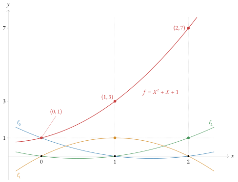
which satisfies f(0)=1, f(1)=3, f(2)=7 as required. 2 plots the three basis polynomials and the interpolant.

Refer to caption
Figure 2: The Lagrange basis polynomials ℓ0, ℓ1, ℓ2 for the nodes 0,1,2 of 5.31, read as functions on ℝ. Each takes the value 1 at its own node and vanishes at the other two, the delta property (4). The interpolant f=1⋅ℓ0+3⋅ℓ1+7⋅ℓ2=X2+X+1 passes through (0,1), (1,3) and (2,7); at the node 0 it meets ℓ0, since y0=1.
Remark 5.32 (The evaluation isomorphism).

Fix d+1 distinct nodes and let V={f∈F[X]:degf≤d}. In the language of the linear-algebra section later in the volume, V is a (d+1)-dimensional vector space over F with basis 1,X,…,Xd, and the evaluation map

ev:V→Fd+1,f⟼(f⁢(x0),…,f⁢(xd)),

is F-linear. Its surjectivity is the existence half of 5.30, and its injectivity the uniqueness half; so ev is a linear isomorphism V≅Fd+1. By the delta property (4), the Lagrange basis {ℓi} is the basis of V matched to the standard coordinates of Fd+1: the polynomial with prescribed values (y0,…,yd) has coordinates (y0,…,yd) in the basis {ℓi}. Conversion between a polynomial’s coefficient representation and its evaluation representation underlies fast polynomial arithmetic via the fast Fourier transform, treated with the roots of unity later in the volume, and the evaluation-domain encodings used throughout Halo 2.

Remark 5.33 (The vanishing polynomial).

Alongside the Lagrange basis, the node set {x0,…,xd} determines its vanishing polynomial

Z⁢(X)=∏i=0d(X−xi),

the unique monic polynomial of degree d+1 vanishing at every node. A polynomial g vanishes on the whole node set if and only if Z∣g. One direction is immediate from 5.16. For the other, apply the factor theorem repeatedly: g(x0)=0 gives g=(X−x0)g1; evaluating at x1≠x0 gives 0=(x1−x0)g1(x1), so g1(x1)=0 since F has no zero divisors, and g1=(X−x1)g2; continuing through the remaining nodes strips off one linear factor per node. The repetition requires the nodes to be distinct, so that the linear factors X−xi are pairwise coprime. A proof system uses the Lagrange basis and the vanishing polynomial to argue that a committed polynomial agrees with prescribed values on an evaluation domain.

5.8 Multiplicity and the formal derivative

A linear factor may divide a polynomial more than once, as in X2−2X+1=(X−1)2. This subsection defines the multiplicity of a root, bounds the number of roots counted with multiplicity, and detects repeated roots with a derivative defined without limits.

Definition 5.34 (Multiplicity of a root).

Let f∈F[X] be nonzero and let α∈F be a root of f. The multiplicity multα(f) is the largest integer m≥1 with (X−α)m∣f. A root of multiplicity 1 is simple; a root of multiplicity at least 2 is repeated (or multiple).

The largest such m exists: the powers (X−α)m have strictly increasing degrees, so only finitely many can divide the fixed f, and at least one does by the factor theorem. In an equivalent characterisation, m=multα(f) holds exactly when f=(X−α)mg with g(α)≠0. Writing f=(X−α)mg with m maximal forces g(α)≠0, else the factor theorem would split a further factor X−α off g; conversely, if f=(X−α)mg with g(α)≠0, then (X−α)m+1∣f would give (X−α)mg=(X−α)m+1h, and cancelling (5.9) g=(X−α)h, making α a root of g.

The number of roots counted with multiplicity is also bounded by the degree; the proof uses the following lemma.

Lemma 5.35 (Coprime factors multiply).

Let f1,…,fr∈F[X] be pairwise coprime (gcd(fi,fj)=1 for i≠j) and suppose each fi divides f. Then f1f2⋯fr∣f.

Proof.

First let r=2, and write f=f1u=f2v. Bézout (3) gives sf1+tf2=1, so

f=s⁢f1⁢f+t⁢f2⁢f=s⁢f1⁢(f2⁢v)+t⁢f2⁢(f1⁢u)=f1⁢f2⁢(s⁢v+t⁢u),

and f1f2∣f. For r>2, induct: by hypothesis f1⋯fr−1∣f, and the product f1⋯fr−1 is coprime to fr—a nonconstant common divisor would have a monic irreducible factor (5.28), which by Euclid’s lemma (5.25(2)) would divide some fi with i<r as well as fr, contradicting gcd(fi,fr)=1. The case r=2 then applies. □

Proposition 5.36 (Counting roots with multiplicity).

Let f∈F[X] be nonzero of degree d, with all its distinct roots α1,…,αr∈F of multiplicities m1,…,mr. Then

f=(X−α1)m1⁢⋯⁢(X−αr)mr⁢g

for some g∈F[X] with no roots in F, and ∑imi≤d. The number of roots counted with multiplicity is thus at most d, with equality if and only if f splits into linear factors over F.

Proof.

We first check that the powers (X−αi)mi are pairwise coprime. Each X−αi is monic irreducible (degree 1), and by unique factorisation the monic divisors of (X−αi)mi are exactly the powers (X−αi)e with 0≤e≤mi. For i≠j the only monic polynomial that is simultaneously a power of X−αi and of X−αj is 1, since X−αi=X−αj would force αi=αj; so gcd((X−αi)mi,(X−αj)mj)=1.

Each (X−αi)mi divides f by the definition of multiplicity, so 5.35 gives f=(X−α1)m1⋯(X−αr)mrg. Maximality of each mi gives g(αi)≠0: a further factor X−αi inside g would raise the multiplicity. Nor has g any other root: a root β of g is a root of f, hence one of the αi. Taking degrees with (2),

m1+⋯+mr+deg⁡g=d,

so ∑imi≤d, with equality precisely when degg=0, that is, when f is a constant times a product of linear factors. □

Definition 5.37 (Formal derivative).

The formal derivative is the map D:F[X]→F[X] defined on f=∑i=0naiXi by

f′=D⁢f=∑i=1ni⁢ai⁢Xi−1=a1+2⁢a2⁢X+⋯+n⁢an⁢Xn−1,

where the coefficient iai means ai added to itself i times in F—that is, ai multiplied by the image of the integer i under the canonical map ℤ→F (4.30). No limits are involved: the definition is formal and algebraic, valid over any field, and is introduced for one purpose, to detect repeated roots without appeal to analysis.

Proposition 5.38 (Rules of formal differentiation).

For all f,g∈F[X], c∈F, α∈F, and m≥1:

  1. 1.

    (Linearity.) (f+g)′=f′+g′ and (cf)′=cf′.

  2. 2.

    (Product rule.) (fg)′=f′g+fg′.

  3. 3.

    (Power rule.) ((X−α)m)′=m(X−α)m−1.

Proof.

(1) Linearity is immediate from the coordinatewise definition of D, which is linear in the coefficients.

(2) Both sides are bilinear in the pair (f,g): by part (1), each is linear in f with g fixed and linear in g with f fixed. It therefore suffices to verify the identity on monomials f=Xa, g=Xb, since every polynomial is a linear combination of monomials and the general case follows by expanding f=∑auaXa, g=∑bvbXb and applying the monomial case termwise. On monomials,

(Xa⁢Xb)′=(Xa+b)′=(a+b)⁢Xa+b−1=a⁢Xa−1⁢Xb+Xa⁢b⁢Xb−1=(Xa)′⁢Xb+Xa⁢(Xb)′,

with the convention that a term carrying the integer coefficient 0 (the case a=0 or b=0) is the zero polynomial.

(3) Induct on m. The base is (X−α)′=1. For the step, the product rule gives

((X−α)m)′ =((X−α)⁢(X−α)m−1)′
=(X−α)m−1+(X−α)⁢(m−1)⁢(X−α)m−2
=m⁢(X−α)m−1.∎

The proof of part (3) of the next theorem needs a repeated root in an extension field not given in advance. The following lemma constructs that extension by applying the quotient construction of Example 4.22 to polynomial rings; its proof transposes the argument that made ℤ/pℤ a field (4.26) from ℤ to F[X].

Lemma 5.39 (Adjoining a root).

Let h∈F[X] be irreducible. Then the quotient ring K=F[X]/(h) is a field; the map a↦a+(h) embeds F into K as a subfield, so that K is an extension of F; and the class α=X+(h) is a root of h in K.

Proof.

The principal ideal (h)=hF[X] is an ideal of the commutative ring F[X] (Example 4.18(2)), so K is a commutative ring under the coset operations (4.20). Its identity is not zero: 1+(h)=0+(h) would say h∣1, impossible since a factorisation 1=hk has degree degh+degk=0 by (2), while degh≥1.

Every nonzero class is a unit. Let f+(h)≠0+(h), i.e. h∤f. The gcd gcd(h,f) is then a monic divisor of the irreducible h other than its monic associate, hence equals 1, exactly as in the proof of 5.25(2); Bézout’s identity (3) supplies s,t∈F[X] with sf+th=1, and reducing modulo (h) gives (s+(h))(f+(h))=1+(h). So K is a field.

The map ι(a)=a+(h) on constants preserves sums, products, and 1 directly from the coset operations of 4.19, and it is injective: ι(a)=0 with a≠0 would make h divide a nonzero constant, again impossible by degrees. We identify F with its image, making K an extension field of F.

Finally, write h=∑iciXi and compute in K:

h⁢(α)=∑iι⁢(ci)⁢(X+(h))i=(∑ici⁢Xi)+(h)=h+(h)=0+(h),

so α is a root of h in K. □

Theorem 5.40 (Derivative test for repeated roots; separability).

Let f∈F[X] be nonzero and α∈F.

  1. 1.

    The element α is a repeated root of f—a root of multiplicity at least 2—if and only if f(α)=0 and f′(α)=0.

  2. 2.

    If f has a repeated root in F, then gcd(f,f′)≠1.

  3. 3.

    Call f separable if it has no repeated root in any field containing F. Then f is separable if and only if gcd(f,f′)=1 in F[X].

Proof.

(1) Let α be a root of multiplicity m≥1 and write f=(X−α)mg with g(α)≠0. The product and power rules give

f′=m⁢(X−α)m−1⁢g+(X−α)m⁢g′=(X−α)m−1⁢[m⁢g+(X−α)⁢g′].

If m=1, the first factor is 1 and evaluating at α gives f′(α)=1⋅g(α)=g(α)≠0: a simple root of f is not a root of f′. If m≥2, then (X−α)m−1 divides f′ and vanishes at α, so f′(α)=0. Together with the factor theorem for f(α)=0, this proves the equivalence.

(2) A repeated root α∈F is a common root of f and f′ by (1), so the factor theorem puts the common factor X−α into both, and (X−α)∣gcd(f,f′).

(3) The argument rests on the fact that gcds are stable under field extension: for an extension field K of F (4.25), the Euclidean algorithm of 5.23 run on f,f′∈F[X] uses only field operations on their coefficients, which lie in F; run inside K[X] on the same inputs it produces the identical quotients and remainders. Hence the gcd computed in K[X] equals the gcd computed in F[X].

Suppose gcd(f,f′)=1 in F[X], and let K⊇F be any extension. By stability, gcd(f,f′)=1 in K[X] as well, so by (2) applied over K, the polynomial f has no repeated root in K: f is separable.

Conversely, suppose d=gcd(f,f′) is nonconstant; we exhibit a repeated root in some extension. Let h be a monic irreducible factor of d (5.28), and let K=F[X]/(h) be the extension field supplied by 5.39, in which h has a root α. The polynomial h divides d, which divides both f and f′; evaluating the factorisations at α (5.16) gives f(α)=f′(α)=0. By (1), applied over K, the element α is a repeated root of f in K: f is not separable. □

Remark 5.41 (Formal derivatives in positive characteristic).

The integer coefficient i in f′=∑iiaiXi−1 is interpreted in F, and may vanish there. Over a field of characteristic p—where p=0 in F, p prime, the setting of 𝔽p and 𝔽q (4.30)—the derivative of Xp is pXp−1=0. Thus f=Xp−1 over 𝔽p has f′=0 and gcd(f,f′)=gcd(f,0)=f≠1; correspondingly,

Xp−1=(X−1)pin ⁢𝔽p⁢[X],

a factorisation the finite-fields section establishes through the freshman’s-dream identity (a+b)p=ap+bp of characteristic p (6.14, applied to (X+(−1))p together with (−1)p=−1 in every 𝔽p): a single root 1 of multiplicity p. Arguments over the finite fields of Orchard must account for this characteristic-p behaviour.

5.9 Polynomials versus polynomial functions

This subsection determines when a polynomial may be identified with the function it induces.

Definition 5.42 (Polynomial function).

Every f∈F[X] induces a polynomial function

f~:F→F,α⟼f⁢(α).

The assignment f↦f~ is a ring homomorphism from F[X] to the ring FF of all functions F→F under pointwise operations ((u+v)(α)=u(α)+v(α) and (uv)(α)=u(α)v(α)), by 5.16 applied at every point.

Proposition 5.43 (When formal equals functional).

Let f,g∈F[X].

  1. 1.

    If F is infinite, then f~=g~ as functions implies f=g as polynomials. Equivalently, f↦f~ is injective, and polynomials over an infinite field may be identified with polynomial functions.

  2. 2.

    If F is finite, the map is not injective. Over 𝔽p, the nonzero polynomial Xp−X induces the zero function, since Fermat’s little theorem (Corollary 3.32) gives αp=α for every α∈𝔽p.

Proof.

(1) Let h=f−g, so that h~ is the zero function: h vanishes at every point of the infinite set F. Were h nonzero of degree d, it would have at most d roots (5.18), yet it has infinitely many—a contradiction. Hence h=0.

(2) Let F be finite, with q=|F| elements, and consider the vanishing-polynomial witness

w⁢(X)=∏α∈F(X−α),

a monic polynomial of degree q—in particular nonzero as a formal object—which vanishes at every point of F by construction. Thus w~=0~ while w≠0: the map f↦f~ identifies distinct polynomials. Over F=𝔽p the witness specialises to Xp−X: by Fermat’s little theorem every element of 𝔽p is a root of the monic degree-p polynomial Xp−X, so 5.36 factors it as ∏α∈𝔽p(X−α)—the p distinct linear factors exhaust the degree—and Xp−X induces the zero function despite having degree p≥1. □

Remark 5.44 (Why polynomials are defined formally).

Part (2) of 5.43 is the reason polynomials are defined as coefficient sequences and not as functions. Cryptography works over finite fields, where the functional view loses information: the polynomials X and Xp induce the same function on 𝔽p, yet have degrees 1 and p. The security of polynomial commitment schemes rests on the degree, a property of the formal object invisible to the induced function over a finite field. A prover commits to a low-degree formal polynomial, and the verifier tests it by evaluation. The Schwartz–Zippel lemma quantifies the gap between agreement at the tested points and identity to the claimed formal polynomial.

5.10 The Schwartz–Zippel lemma

To draw α uniformly at random from a finite nonempty set S means to select each element with equal likelihood 1/|S|; the probability of an event is then the fraction of elements of S producing it, so that Pr[f(α)=0]=|{α∈S:f(α)=0}|/|S|. The theorem needs only this counting case; probability is developed later in the volume.

Theorem 5.45 (Univariate Schwartz–Zippel).

Let f∈F[X] be nonzero of degree at most d, let S⊆F be finite and nonempty, and let α be drawn uniformly at random from S. Then

Pr⁡[f⁢(α)=0]≤d|S|. (5)

More generally, if f,g∈F[X] are distinct, each of degree at most d, then Pr[f(α)=g(α)]≤d/|S|.

Proof.

By 5.18, the nonzero f has at most d roots in F, hence at most d in the subset S. Under the uniform draw,

Pr⁡[f⁢(α)=0]=|{α∈S:f⁢(α)=0}||S|≤d|S|.

For the general form, apply this to h=f−g, which is nonzero and has degree at most d by (1), noting that f(α)=g(α) exactly when h(α)=0. □

Remark 5.46 (Polynomial identity testing).

Inequality (5) is the probabilistic refinement of 5.20: a single random evaluation point detects unequal polynomials of degree at most d, except with probability at most d/|S|. With |S| exponentially large (S=𝔽q with q≈2254, the 255-bit fields underlying Orchard) and d polynomially bounded, the failure probability is exponentially small, hence negligible, a term given its precise asymptotic meaning later in the volume. The bound is the soundness argument for polynomial identity testing, and hence for the polynomial commitment schemes and arithmetisation checks of Halo 2, which verify a purported polynomial identity by evaluating both sides at a random challenge and comparing the results.

Remark 5.47 (Multivariate generalisation).

The full Schwartz–Zippel lemma extends to polynomials in several indeterminates f∈F[X1,…,Xn]: a nonzero polynomial of total degree d—the largest sum of exponents i1+⋯+in over the monomials with nonzero coefficient—vanishes at a uniformly random point of Sn with probability at most d/|S|. The univariate case proved here is the base case of the multivariate inductive proof and the only version the later volumes invoke directly. Where an identity in several random challenges arises, for instance in a permutation argument drawing a pair of challenges (β,γ), the multivariate bound applies and follows from the univariate lemma applied once per variable.

Over a 255-bit field 𝔽q, distinct polynomials f and g of degree at most d agree on a uniformly random challenge α∈𝔽q with probability at most d/q≈d⋅2−254, astronomically small even with d in the millions.