III Halo 2 Guide: The Halo 2 proof system, from arithmetisation to recursion 1 Introduction 3 The inner-product polynomial commitment

2 Arithmetisation: from a computation to committed polynomials

This section carries the running example of §1 — the prover knows $x=3$ with $x^{3}+x+5=35$ over $\mathbb{F}_{97}$ — from a computation to a handful of polynomials that a verifier can query at one point, toy first and general second. It ends with the property the argument has not yet provided: that the queried polynomials are fixed before the evaluation point is chosen.

2.1 From computation to a grid of constraints

The verifier cannot evaluate the computation without the witness. Arithmetisation dismantles the computation into local facts, each involving only a handful of values, arranged so that “every local fact holds and the values are consistently shared” is equivalent to “the whole computation ran correctly”. The dialect of arithmetisation Halo 2 uses is called PLONKish; §2.5 defines it once the toy has shown what it generalises.

Execution trace.

Evaluate $x^{3}+x+5$ the way a machine would, naming every intermediate value:

x^{2}=x\cdot x,\qquad x^{3}=x^{2}\cdot x,\qquad s=x^{3}+x,\qquad s+5=35.

Four elementary operations, two multiplications and two additions, and each becomes one row of a table. A row has three wires $a, b, c$ (two inputs and an output) and a bank of five selectors $q_{M},q_{L},q_{R},q_{O},q_{C}$ that switch on whichever gate the row performs. The universal gate equation, imposed at every row, is

q_{M}\,a\,b+q_{L}\,a+q_{R}\,b+q_{O}\,c+q_{C}+\mathrm{PI}=0,

(1)

where $\mathrm{PI}$ carries the negated public input on that row (here $-35$ , for the target $35$ ). A multiplication gate $a\cdot b=c$ is the choice $q_{M}=1$ , $q_{O}=-1$ and the rest zero; an addition gate $a+b=c$ is $q_{L}=q_{R}=1$ , $q_{O}=-1$ . Filling in the four operations gives the execution trace of Table 1. Definition 2.7 generalises this fixed selector bank to arbitrary custom gates and lookup arguments (the halo2 book’s PLONKish Arithmetization chapter); §4 gives the form of the Action circuit’s gates, and one in full, under “From statement to circuit: arithmetisation in practice”.

row	$a$	$b$	$c$	$q_{M}$	$q_{L}$	$q_{R}$	$q_{O}$	$q_{C}$	$\mathrm{PI}$	gate performed
$0$	$3$	$3$	$9$	$1$	$0$	$0$	$-1$	$0$	$0$	$x\cdot x=x^{2}$
$1$	$9$	$3$	$27$	$1$	$0$	$0$	$-1$	$0$	$0$	$x^{2}\cdot x=x^{3}$
$2$	$27$	$3$	$30$	$0$	$1$	$1$	$-1$	$0$	$0$	$x^{3}+x=s$
$3$	$30$	$0$	$0$	$0$	$1$	$0$	$0$	$5$	$-35$	$s+5=35$

Table 1: The execution trace for

x=3

, all entries in

\mathbb{F}_{97}

(so

-1=96

and

-35=62

). Every row satisfies the gate equation (1): row

0

reads

1\cdot 3\cdot 3+(-1)\cdot 9=0

and row

3

reads

1\cdot 30+5+(-35)=0

. The selector columns

q_{\bullet}

are fixed circuit data and

\mathrm{PI}

is the negated public input, both known to the verifier; the wires

a, b, c

are the prover’s advice, her secret trace.

Copy constraints.

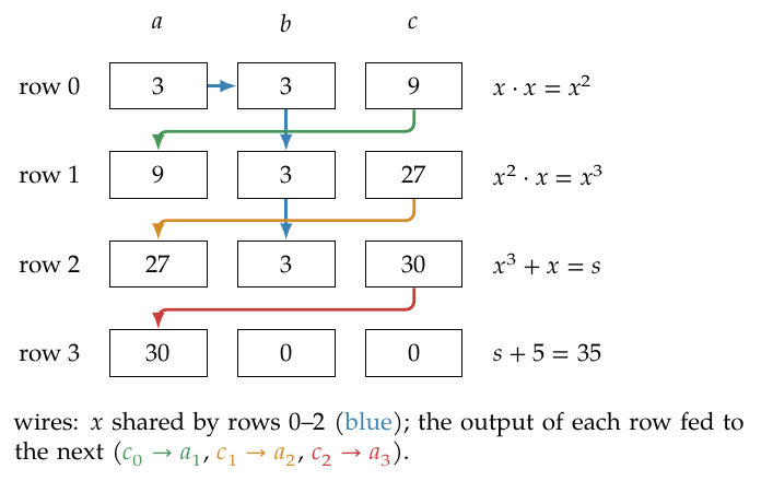
The table as printed does not yet encode the computation. Nothing forces the $x$ in row $0$ to equal the $x$ in rows $1$ and $2$ , nor the output $x^{2}=9$ of row $0$ to be the input of row $1$ . A cheating prover could put $x=3$ in row $0$ and $x=8$ in row $2$ and satisfy each gate in isolation without the rows forming one computation. The missing assertions are that certain cells are equal, the copy constraints (also called equality constraints):

\underbrace{a_{0}=b_{0}=b_{1}=b_{2}}_{\text{all are }x=3},\qquad\underbrace{c_% {0}=a_{1}}_{x^{2}=9},\qquad\underbrace{c_{1}=a_{2}}_{x^{3}=27},\qquad% \underbrace{c_{2}=a_{3}}_{s=30},

where $a_{j}$ denotes the cell of column $a$ in row $j$ . Figure 2 draws them as wires. They turn a list of unrelated gates into a single dataflow; enforcing them is an argument in its own right, the permutation argument of §2.6.

Refer to caption — Figure 2: The four-row trace of Table 1 with the copy constraints drawn as wires. Each wire colour is one class of cells that must hold a single value: the blue wire ties the four occurrences of $x$ , and the three coloured wires carry each row’s output $c_{j}$ into the next row’s input $a_{j+1}$ . The gates check rows; the wires make the rows one computation.

Satisfiability of the grid.

The claim is now equivalent to a purely combinatorial assertion: there exist values for the advice cells $a, b, c$ such that (i) every row satisfies the gate equation (1) with the fixed selectors, and (ii) every copy constraint holds. Knowing $x$ is exactly knowing how to fill the advice columns. The verifier knows the fixed columns and the public input; the prover must convince him that satisfying advice exists while revealing none of it. Everything that follows is machinery for doing precisely that.

2.2 From the grid to polynomials

The grid has finitely many rows, and the aim is a statement about all rows at once that the verifier can check at one point. A polynomial of degree less than $n$ is determined by its values at $n$ distinct points (Math Guide, §“Lagrange interpolation”), and the rest of the section relies on this.

An index set for the rows.

The table has $n=4$ rows, and four distinct field elements must name them. The chosen four are the $4$ th roots of unity. A primitive $n$ -th root of unity is an element $\omega$ with $\omega^{n}=1$ and no smaller positive power equal to $1$ (Math Guide, §“Roots of unity”), and the evaluation domain it generates is $H=\{\omega^{0},\dots,\omega^{n-1}\}$ , a multiplicative subgroup of $\mathbb{F}^{\times}$ of order $n$ (Math Guide, §“The evaluation domain $H$ and its vanishing polynomial”). In $\mathbb{F}_{97}$ take $\omega=22$ : then $\omega^{2}=96=-1$ and $\omega^{4}=1$ , so

H=\{\omega^{0},\omega^{1},\omega^{2},\omega^{3}\}=\{1,22,96,75\}=\{1,22,-1,-22\},

and row $i$ lives at the point $\omega^{i}$ . Roots of unity are chosen because they form a cyclic group: the row after $\omega^{i}$ is $\omega\cdot\omega^{i}$ , so reading a column at the next row is evaluating its polynomial at $\omega X$ ; the polynomial vanishing on $H$ is $X^{n}-1$ ; and interpolation over $H$ is a fast Fourier transform (Math Guide, §“The fast Fourier transform”). The gate check of this subsection alone would hold over any four distinct points.

Columns become polynomials.

Each column of the table is four numbers, one per row. Interpolate: for the advice column $a$ there is a unique polynomial $a(X)$ of degree $<4$ with

a(\omega^{0})=3,\quad a(\omega^{1})=9,\quad a(\omega^{2})=27,\quad a(\omega^{3% })=30

(Math Guide, §“Lagrange interpolation”), and likewise $b(X)$ , $c(X)$ , the publicly known selector polynomials $q_{M},q_{L},q_{R},q_{O},q_{C}$ and the public-input polynomial $\mathrm{PI}$ , each of degree $<4$ . Computed over $\mathbb{F}_{97}$ , the nine interpolants are

$\displaystyle a(X)$	$\displaystyle=90+61X+22X^{2}+24X^{3},$	$\displaystyle q_{M}(X)$	$\displaystyle=49+19X+30X^{3},$
$\displaystyle b(X)$	$\displaystyle=75+32X+25X^{2}+65X^{3},$	$\displaystyle q_{L}(X)$	$\displaystyle=49+78X+67X^{3},$
$\displaystyle c(X)$	$\displaystyle=65+16X+3X^{2}+22X^{3},$	$\displaystyle q_{R}(X)$	$\displaystyle=73+24X+73X^{2}+24X^{3},$
$\displaystyle\mathrm{PI}(X)$	$\displaystyle=64+50X+33X^{2}+47X^{3},$	$\displaystyle q_{O}(X)$	$\displaystyle=72+54X+24X^{2}+43X^{3},$
$\displaystyle q_{C}(X)$	$\displaystyle=74+76X+23X^{2}+21X^{3},$

and each returns its column at the rows: $b$ takes the values $(3,3,3,0)$ on $H$ , $q_{O}$ the values $(96,96,96,0)$ , and $\mathrm{PI}$ the values $(0,0,0,62)$ . Interpolation is thus a bijection between columns of four values and polynomials of degree $<4$ : the encoding loses no information.

The gate polynomial.

Assemble the left-hand side of the gate equation (1) with the polynomials in place of the per-row numbers.

Theorem 2.1 (The gate polynomial).

Let

G(X):=q_{M}(X)\,a(X)\,b(X)+q_{L}(X)\,a(X)+q_{R}(X)\,b(X)+q_{O}(X)\,c(X)+q_{C}(% X)+\mathrm{PI}(X).

(2)

Then $\deg G\leq 9$ , and $G(\omega^{i})=0$ for every row $i$ if and only if every gate of the trace is satisfied.

Proof.

The term $q_{M}ab$ multiplies three polynomials of degree at most $3$ , and every other term has degree at most $6$ , so $\deg G\leq 9$ . Evaluate $G$ at the label $\omega^{i}$ of row $i$ : each column polynomial returns that row’s value there, so $G(\omega^{i})$ is exactly the left-hand side of (1) for row $i$ . It is zero precisely when gate $i$ holds, and the conjunction over $i$ gives the claim. □

For the honest trace,

G(X)=36+27X+54X^{2}+50X^{3}+77X^{4}+24X^{5}+43X^{6}+47X^{7}+81X^{8}+46X^{9},

of degree exactly $9$ , and it vanishes at all four points of $H$ by construction. “Every gate is satisfied” has become “ $G$ vanishes on $H$ ”; the copy constraints remain separate. Four separate checks are now one statement about one polynomial.

2.3 From vanishing to a single identity

The condition “ $G$ vanishes on $H$ ” is still a statement about four points. This subsection replaces it by a polynomial identity that refers to no individual row.

The vanishing polynomial.

The vanishing polynomial of $H$ is the monic polynomial (leading coefficient $1$ ) whose roots are exactly the points of $H$ ,

Z_{H}(X):=\prod_{i=0}^{3}(X-\omega^{i})=X^{4}-1,

where the closed form $X^{n}-1$ holds for every evaluation domain of order $n$ (Math Guide, §“The evaluation domain $H$ and its vanishing polynomial”): each $\omega^{i}$ is a root of $X^{n}-1$ , there are $n$ distinct ones, and comparing leading coefficients finishes. The closed form lets both parties evaluate $Z_{H}$ at any point with $O(\log n)$ multiplications.

Theorem 2.2 (Gate satisfaction is a quotient).

Every gate of the trace holds if and only if there is a polynomial $t(X)$ with $G(X)=t(X)\,Z_{H}(X)$ .

Proof.

By Theorem 2.1, every gate holds if and only if $G$ vanishes on $H$ . The factor theorem (Math Guide, §“Roots and the factor theorem”) gives $G(\omega^{i})=0$ if and only if $(X-\omega^{i})\mid G$ ; and because the four roots are distinct, $G$ vanishes at all of them if and only if the product of the four linear factors divides $G$ (Math Guide, §“Lagrange interpolation”, its remark on the vanishing polynomial: a polynomial vanishes on a set of distinct nodes if and only if the product of the corresponding linear factors divides it). Thus

G\text{ vanishes on }H\iff(X-\omega^{i})\mid G\text{ for each }i\iff Z_{H}(X)% \mid G(X),

(3)

and divisibility is the existence of the quotient $t$ . □

Satisfaction of the gate constraints is precisely the existence of $t$ ; correct wiring still requires the copy constraints. For the honest trace the division comes out even: $G$ has degree $9$ , $Z_{H}$ has degree $4$ , and

t(X)=\frac{G(X)}{X^{4}-1}=61+70X+43X^{2}+47X^{3}+81X^{4}+46X^{5}

is a polynomial of degree $5$ with remainder zero, as it must be.

Example 2.3 (Why a cheat cannot produce $t$ ).

Suppose the advice is wrong: some gate fails. Then $G$ does not vanish on all of $H$ , so by (3) $Z_{H}$ does not divide $G$ , and no polynomial $t$ satisfies $G=t\,Z_{H}$ . The dividing line is exact: the quotient exists if and only if every gate is satisfied. Concretely, take a prover who claims $x^{2}=10$ and writes $c_{0}=10$ in row $0$ of Table 1 instead of $9$ . Row $0$ ’s gate now reads $3\cdot 3-10=-1\neq 0$ , so the tampered gate polynomial $G^{*}$ has $G^{*}(\omega^{0})=-1=96$ while still vanishing at the other three rows:

G^{*}(X)=54+10X+43X^{2}+74X^{3}+83X^{4}+65X^{5}+78X^{6}+47X^{7}+81X^{8}+46X^{9}.

Dividing $G^{*}$ by $Z_{H}$ with remainder (Math Guide, §“Division with remainder”) gives the quotient $t^{*}(X)=67+14X+78X^{2}+47X^{3}+81X^{4}+46X^{5}$ and a nonzero remainder. This Euclidean quotient is an illustrative choice for $t^{*}$ , not a claim that it maximises the cheat’s chances. Whatever $t^{*}$ she offers as the quotient, the gap polynomial $D(X):=G^{*}(X)-t^{*}(X)\,Z_{H}(X)$ is nonzero, since $Z_{H}$ does not divide $G^{*}$ . For the Euclidean quotient $D$ is the remainder,

D(X)=24\,(1+X+X^{2}+X^{3}),

(4)

of degree $3$ . The identity $G^{*}=t^{*}\,Z_{H}$ is false, $D$ is the difference of its two sides, and §2.4 shows how the verifier detects $D\neq 0$ .

2.4 Why checking one random point is a proof

The prover wishes to convince the verifier that $G(X)=t(X)\,Z_{H}(X)$ as polynomials, with $G$ built from her secret advice. The verifier does not read the polynomials: they encode the witness, and reading them would cost time at least linear in the number of rows. Instead, the two run a four-step protocol. A commitment is, for now, a short string that fixes a value without revealing it (Crypto Guide, §“Commitment schemes”); §2.9 says what a commitment to a polynomial must do and which one Halo 2 uses.

Construction 2.4 (The random-point check).

1.

The prover commits to her polynomials $a, b, c$ and to the quotient $t$ ; the selector and public-input polynomials the verifier already knows.
2.

The verifier picks a point $z\in\mathbb{F}$ uniformly at random and sends it.
3.

The prover opens her commitments at $z$ : she returns the field elements $a(z),b(z),c(z),t(z)$ together with short proofs that these are the true evaluations of the committed polynomials.
4.

The verifier forms $G(z)$ from the openings and the self-evaluated public polynomials via (2), computes $Z_{H}(z)=z^{4}-1$ , and checks the single field equation

$G(z)\overset{?}{=}t(z)\,Z_{H}(z).$ (5)

He accepts if and only if (5) holds.

The honest case (completeness).

If the prover is honest then $G=t\,Z_{H}$ holds as polynomials, hence at every point, hence at $z$ . With the honest trace and the draw $z=20$ ,

Z_{H}(20)=20^{4}-1=46,\qquad t(20)=67,\qquad G(20)=75=67\cdot 46=t(20)\,Z_{H}(% 20),

and the verifier accepts. He accepts every time, for every $z$ .

The dishonest case (soundness).

Soundness rests on the fact that a nonzero polynomial of low degree has few roots.

Theorem 2.5 (Soundness of the random-point check).

Suppose the trace is invalid, so that the prover’s gate polynomial $G^{*}$ does not vanish on all of $H$ , and let $t^{*}$ be any polynomial she commits to as the quotient. Set $D(X):=G^{*}(X)-t^{*}(X)\,Z_{H}(X)$ . Then $D$ is a nonzero polynomial, and if the prover’s polynomials $a, b, c$ (which determine $G^{*}$ ) and $t^{*}$ are fixed before $z$ is drawn and the verifier receives their true evaluations at $z$ ,

\mathrm{Pr}_{z}\bigl{[}\text{the verifier accepts}\bigr{]}=\mathrm{Pr}_{z}% \bigl{[}D(z)=0\bigr{]}\leq\frac{\deg D}{|\mathbb{F}|}.

Proof.

Were $D$ the zero polynomial, $G^{*}=t^{*}\,Z_{H}$ would be divisible by $Z_{H}$ and so, by (3), vanish on all of $H$ , which it does not. Hence $D\neq 0$ for every choice of $t^{*}$ . By hypothesis $a, b, c$ and $t^{*}$ , and with them $G^{*}$ and $D$ , are fixed before $z$ is drawn (the verifier never receives $G^{*}$ itself; from the evaluations at $z$ he reconstructs only the single number $G^{*}(z)$ ). The check (5) passes at $z$ exactly when $G^{*}(z)-t^{*}(z)\,Z_{H}(z)=D(z)=0$ , that is, exactly when $z$ is a root of $D$ . A nonzero polynomial of degree at most $\deg D$ has at most $\deg D$ roots, so a uniformly random $z$ is one of them with probability at most $\deg D/|\mathbb{F}|$ (Math Guide, §“The Schwartz–Zippel lemma”). □

The bound $\deg D/|\mathbb{F}|$ is negligible when $|\mathbb{F}|$ is exponential in the security parameter and $\deg D$ is polynomial in it. The verifier does not recompute the trace; he tests one polynomial identity at one random point.

Example 2.6 (The random-point check on the toy).

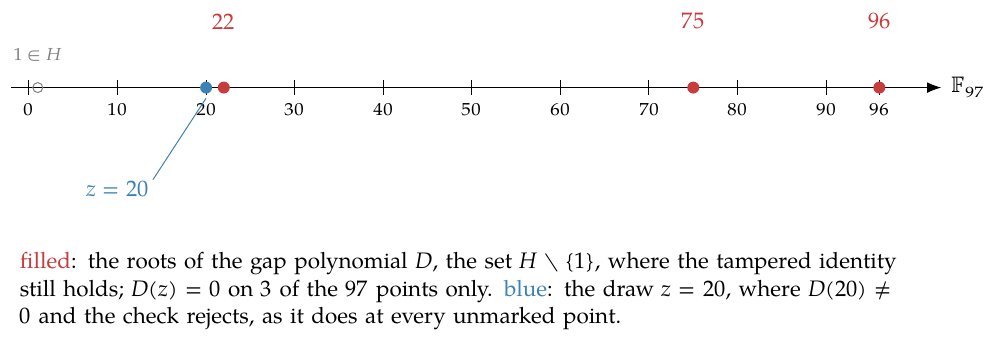
For the $x^{2}=10$ cheat of Example 2.3, $D(X)=24(1+X+X^{2}+X^{3})$ has degree $3$ and so at most $3$ roots; in $\mathbb{F}_{97}$ its roots are exactly $\{22,96,75\}$ , the three rows where the tampered gate still held (Figure 3). This particular quotient choice slips past only if the random $z$ lands in that three-element set:

\mathrm{Pr}[\text{cheat accepted}]=\frac{3}{97}.

At the actual draw $z=20\notin\{22,96,75\}$ the openings give $G^{*}(20)=20$ but $t^{*}(20)\,Z_{H}(20)=64$ ; since $20\neq 64$ , the verifier rejects.

Scale.

The fraction $3/97$ is large only because the field is a toy, and it concerns one particular quotient; the next paragraph bounds every cheat by $11/97$ . What such a term means at the deployed field size is the scale caveat of §1.2.

Bounding the degree.

The argument needs $\deg D$ small relative to $|\mathbb{F}|$ , otherwise “ $\deg D$ roots out of $|\mathbb{F}|$ ” is no constraint at all. The commitment scheme enforces a degree bound on every committed polynomial (Crypto Guide, §“Polynomial commitment schemes”), so the prover cannot commit to a $t^{*}$ of unbounded degree. The bound follows the degree the commitment admits, not the honest degree. The wires are committed at degree below $n=4$ , so $\deg G^{*}\leq 9$ ; committed as the two pieces of degree below $n$ that the deployed rule below prescribes, $t^{*}$ has degree at most $7$ , so $\deg(t^{*}Z_{H})\leq 11$ and $\deg D\leq 11$ . Every cheat is therefore accepted with probability at most $11/97$ , and some cheat attains it, where the illustrative quotient reaches $3/97$ : the $t^{*}$ of degree $7$ that agrees with $G^{*}/Z_{H}$ at the eight points $2,\dots,9$ gives $D$ the eleven roots $2,\dots,9,22,75,96$ . This is why a circuit’s gates are kept to low degree, and why the quotient $t$ , of degree $5$ here and up to a few times $n$ in general, is split into degree-bounded pieces. In the deployed system the quotient is cut into pieces of degree below $n$ , each committed separately (the halo2 book’s Vanishing argument chapter); “The complete Halo 2 protocol” in §4 gives the count.

2.5 PLONKish arithmetisation

The toy has met every ingredient concretely: an evaluation domain $H$ , a generator $\omega$ , the vanishing polynomial $Z_{H}$ , columns interpolated into polynomials of degree $<n$ , and a gate expressed as a polynomial identity on $H$ . The general object can now be named.

Definition 2.7 (PLONKish constraint system).

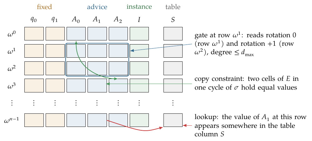
Fix a prime field $\mathbb{F}$ and an integer $k$ with $2^{k}\mid|\mathbb{F}|-1$ , so that $\mathbb{F}^{\times}$ contains a primitive $2^{k}$ -th root of unity $\omega$ (Math Guide, §“Existence over finite fields: the condition $n\mid q-1$ ”), and let $H:=\{\omega^{0},\dots,\omega^{n-1}\}\subset\mathbb{F}^{\times}$ be the multiplicative subgroup of size $n:=2^{k}$ that $\omega$ generates. Its vanishing polynomial is $Z_{H}(X):=X^{n}-1$ , zero exactly on $H$ , so a congruence $p(X)\equiv 0\pmod{Z_{H}(X)}$ means “ $p$ is zero at every row $\omega^{i}$ ”, that is, $Z_{H}\mid p$ . A PLONKish circuit $\mathcal{C}$ over $H$ consists of:

1.

a finite set $\mathrm{Col}$ of columns, each of $n$ cells, one per row, partitioned into fixed columns (preprocessed circuit data, known to both parties), advice columns (the prover’s witness) and instance columns (public input); a cell is an element of $H\times\mathrm{Col}$ , and the circuit assigns every cell of a fixed column its value;
2.

a maximum constraint degree $d_{\max}$ ;
3.

a finite set $R\subset\mathbb{Z}$ of rotations containing $0$ ; a column expression is a polynomial over $\mathbb{F}$ in the values $v(\omega^{r}X)$ for $v\in\mathrm{Col}$ and $r\in R$ , where the value of $v$ at rotation $r$ at row $i$ is the cell of $v$ in row $i+r$ taken modulo $n$ ;
4.

a finite sequence of custom gates $g_{j}=0$ , each $g_{j}$ a column expression of degree at most $d_{\max}$ ;
5.

a set $H_{\mathrm{act}}\subseteq H$ of active rows: all of $H$ in the toy, and in the deployed system the first $u<n$ rows $\omega^{0},\dots,\omega^{u-1}$ , the trailing rows being reserved for a boundary row and blinding (Remark 2.17 fixes $u$ );
6.

a subset $E\subseteq H_{\mathrm{act}}\times\mathrm{Col}$ of equality-constrained cells together with a permutation $\sigma$ of $E$ (a bijection $E\to E$ ) whose cycles, the orbits $\{\kappa,\sigma(\kappa),\sigma^{2}(\kappa),\dots\}$ of the cells $\kappa\in E$ , are the classes of cells required to hold a common value;
7.

a set of lookup arguments, each an input tuple $(A_{0},\dots,A_{m-1})$ of column expressions and a table tuple $(S_{0},\dots,S_{m-1})$ of columns.

An assignment gives every cell a value in $\mathbb{F}$ , the fixed cells their circuit values; write $v_{\kappa}$ for the value of cell $\kappa$ . It is satisfying if every gate vanishes at every row of $H$ (in the deployed system the selectors are zero outside $H_{\mathrm{act}}$ ), $v_{\kappa}=v_{\sigma(\kappa)}$ for every $\kappa\in E$ , and for every lookup and every active row $\omega^{i}$ the tuple $(A_{0}(\omega^{i}),\dots,A_{m-1}(\omega^{i}))$ equals $(S_{0}(\omega^{i^{\prime}}),\dots,S_{m-1}(\omega^{i^{\prime}}))$ for some active row $\omega^{i^{\prime}}$ . The relation $\mathcal{R}_{\mathcal{C}}$ of the circuit is the set of pairs (instance-column values, advice-column values) of the satisfying assignments.

The letter $d$ is reserved, from §3 on, for the length of a committed vector; the constraint degree is therefore written $d_{\max}$ throughout this volume.

Vanilla PLONK as the special case.

The original PLONK system of Gabizon, Williamson and Ciobotaru uses a single fixed five-selector universal gate,

q_{M}(X)\,a(X)\,b(X)+q_{L}(X)\,a(X)+q_{R}(X)\,b(X)+q_{O}(X)\,c(X)+q_{C}(X)+% \mathrm{PI}(X)\equiv 0\pmod{Z_{H}(X)},

with three wire polynomials $a, b, c$ , selector polynomials $q_{M},q_{L},q_{R},q_{O},q_{C}$ and the public-input polynomial $\mathrm{PI}$ , carrying the negated public inputs; the toy’s gate (1) is exactly this gate, with $\mathrm{PI}$ held in an instance column. PLONKish generalises it by permitting designer-chosen gates of higher arity and degree, each switched by its own selector $q_{i}(X)$ , a fixed column that vanishes on the rows where the gate is inactive. In the toy the five selectors are fixed columns, $a, b, c$ are advice, $\mathrm{PI}$ is the instance column, the single gate has degree $3$ and reads rotation $0$ only, and the copy constraints of §2.1 are the equality set $E$ with $\sigma$ cycling each class; there are no lookups until §2.7. Figure 4 shows the general shape.

Columns as committed polynomials.

With the Lagrange basis $\ell_{j}(X)$ of $H$ , defined by $\ell_{j}(\omega^{j})=1$ and $\ell_{j}(\omega^{j^{\prime}})=0$ for $j^{\prime}\neq j$ (Math Guide, §“The Lagrange basis on $H$ ”), a column with cells $v_{0},\dots,v_{n-1}$ is the polynomial $v(X)=\sum_{j}v_{j}\,\ell_{j}(X)$ of degree $<n$ , exactly as the toy’s columns were interpolated in §2.2. The prover commits to each advice polynomial, and the fixed polynomials are committed once for all proofs, with the inner-product polynomial commitment of §3. Every argument that follows — gates, permutation, lookup, vanishing — is a polynomial identity on these committed polynomials, verified by querying them at random points exactly as §2.4 queried $G$ and $t$ .

2.6 Enforcing the wiring: the permutation argument

The copy constraints of §2.1 remain to be enforced. The gate identity of §§2.2–2.4 checks each row separately; it does not assert that $a_{0},b_{0},b_{1},b_{2}$ are the same value $x$ , or that row $1$ ’s input is row $0$ ’s output, and a prover could satisfy every gate with rows that do not form one computation. The permutation argument reduces the equalities to the equality of two products, which is checked at random challenges.

Equalities as a permutation.

Group the cells into the classes that must share a value, $\{a_{0},b_{0},b_{1},b_{2}\}$ , $\{c_{0},a_{1}\}$ , $\{c_{1},a_{2}\}$ , $\{c_{2},a_{3}\}$ , and let $\sigma$ be the permutation of the twelve cells that cycles each class in the order written and fixes $b_{3}$ and $c_{3}$ :

a_{0}\to b_{0}\to b_{1}\to b_{2}\to a_{0},\qquad c_{0}\leftrightarrow a_{1},% \qquad c_{1}\leftrightarrow a_{2},\qquad c_{2}\leftrightarrow a_{3}.

Give every cell a distinct label: the cell in row $j$ of the $a$ -, $b$ -, $c$ -column gets $\omega^{j}$ , $k_{1}\omega^{j}$ , $k_{2}\omega^{j}$ respectively, where $k_{1},k_{2}$ place the three columns in disjoint cosets of $H$ so that no two labels collide. Two cosets of a subgroup are equal or disjoint (Math Guide, §“Cosets and Lagrange’s theorem”), so it suffices that $k_{1}$ , $k_{2}$ and $k_{2}/k_{1}$ all lie outside $H$ ; in $\mathbb{F}_{97}$ take $k_{1}=2$ , $k_{2}=3$ :

H=\{1,22,96,75\},\qquad 2H=\{2,44,95,53\},\qquad 3H=\{3,66,94,31\}.

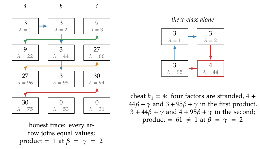
Write $\lambda_{\mathrm{cell}}$ for a cell’s label and $v_{\mathrm{cell}}$ for its value. Asserting “cells in a class are equal” is then equivalent to asserting that the multiset (a finite collection in which an element may occur more than once; two multisets are equal when every element occurs equally often in both) of pairs $\{(v_{\mathrm{cell}},\lambda_{\mathrm{cell}})\}$ is unchanged when each label is replaced by the label of the cell’s image under $\sigma$ : a pair $(v,\lambda)$ moves to $(v,\lambda_{\sigma})$ , and the moved pair was already present exactly when the cell at $\lambda_{\sigma}$ carried the same value $v$ . Figure 5 draws the cycles with their labels. Because labels are distinct, comparing two multisets of pairs is a job for a product: compress each pair to the linear form $v+\beta\,\lambda+\gamma$ with verifier challenges $\beta,\gamma$ , and compare

\prod_{\text{cells}}\bigl{(}v_{\mathrm{cell}}+\beta\,\lambda_{\mathrm{cell}}+% \gamma\bigr{)}\quad\text{against}\quad\prod_{\text{cells}}\bigl{(}v_{\mathrm{% cell}}+\beta\,\lambda_{\sigma(\mathrm{cell})}+\gamma\bigr{)}.

(6)

If the wiring is honest the two products run over the same multiset of factors and agree identically in $\beta,\gamma$ . If a copy constraint is false the difference is a nonzero polynomial in $\beta,\gamma$ , which can still vanish at one particular challenge pair, but only rarely; the converse is probabilistic, not an “if and only if” for fixed challenges. Theorem 2.11 below makes both halves precise.

The running product.

A product over all cells is not a local fact, so the prover commits to a running product: a column $Z_{\mathrm{perm}}$ with $Z_{\mathrm{perm}}(\omega^{0})=1$ whose row $j+1$ equals row $j$ times the ratio of row $j$ ’s factors in (6), numerator over denominator. After the last row the product has run over every cell, and because $\omega^{n}=\omega^{0}$ the row-to-row rule at the last row forces the full product to equal $Z_{\mathrm{perm}}(\omega^{0})=1$ again: the grand product is $1$ exactly when the running product closes its loop. The deployed circuit imposes the rule cross-multiplied, “next row times denominator equals this row times numerator”, not as a field division, so a zero factor never makes the constraint undefined; the prover commits to $Z_{\mathrm{perm}}$ and the verifier checks the boundary value and the row-to-row update at the random point, exactly as he checked the gate identity (the halo2 book’s Permutation argument chapter). The identities are written out in Construction 2.10.

A single wired pair.

Strip the product down to a single wired pair, $c_{0}=a_{1}$ (both should be $9$ ), with labels $\lambda_{c_{0}}=3$ and $\lambda_{a_{1}}=22$ that $\sigma$ swaps. Their factors satisfy

\bigl{(}9+\beta\,\lambda_{c_{0}}+\gamma\bigr{)}\bigl{(}9+\beta\,\lambda_{a_{1}% }+\gamma\bigr{)}=\bigl{(}9+\beta\,\lambda_{a_{1}}+\gamma\bigr{)}\bigl{(}9+% \beta\,\lambda_{c_{0}}+\gamma\bigr{)},

because the shared value $9$ makes the two left-hand factors a mere reordering of the two right-hand ones: the labels may permute under $\sigma$ precisely because the values agree. Now let the prover cheat the copy, $a_{1}=8\neq 9$ . The factor $8+\beta\,\lambda_{a_{1}}+\gamma$ on the left is matched on the right only by $8+\beta\,\lambda_{c_{0}}+\gamma$ , which differs since the labels differ; the two products differ as polynomials in $\beta,\gamma$ . A single unequal value thus leaves a factor without a partner, and the two products differ.

Example 2.8 (The permutation check on the toy).

For the honest trace with $\beta=\gamma=2$ , the ratio of the two products in (6) over all twelve cells is exactly $1$ . Tamper one wire, setting $b_{1}=4$ and so breaking the copy $b_{1}=x=3$ , and the same ratio at the same challenges becomes $61\neq 1$ : the inconsistent dataflow is exposed without any value being revealed.

The general argument.

Halo 2 states the argument for any number of columns, and the statement needs one lemma on two-variable polynomials. The Schwartz–Zippel lemma of the Math Guide (§“The Schwartz–Zippel lemma”) is univariate; that section’s remark on the multivariate generalisation states the several-variable bound without proof, as a consequence of the univariate lemma applied once per variable, and Lemma 2.9 carries out that derivation for two variables.

Lemma 2.9 (Two variables).

Let $P\in\mathbb{F}[\beta,\gamma]$ be nonzero, of degree at most $N$ in each variable separately. For $\beta,\gamma$ drawn independently and uniformly from $\mathbb{F}$ , $\mathrm{Pr}[P(\beta,\gamma)=0]\leq 2N/|\mathbb{F}|$ .

Proof.

Write $P=\sum_{e}c_{e}(\beta)\,\gamma^{e}$ with coefficients $c_{e}\in\mathbb{F}[\beta]$ of degree at most $N$ . Since $P\neq 0$ , some $c_{e_{0}}\neq 0$ , and $c_{e_{0}}(\beta)=0$ with probability at most $N/|\mathbb{F}|$ (Math Guide, §“The Schwartz–Zippel lemma”). When $c_{e_{0}}(\beta)\neq 0$ , the polynomial $P(\beta,\cdot)\in\mathbb{F}[\gamma]$ is nonzero of degree at most $N$ , so it vanishes at the independent uniform $\gamma$ with probability at most $N/|\mathbb{F}|$ . The union bound (Math Guide, §“The union bound and a birthday calculation”) adds the two. □

Construction 2.10 (Permutation argument over $m$ columns).

Let $v_{0}(X),\dots,v_{m-1}(X)$ be the interpolants of the $m$ columns that participate in equality constraints, and let $N=mn$ be the number of participating cells. Label the cell $(i,j)$ (column $i$ , row $j$ ) by $\delta_{i}\,\omega^{j}$ , where $\delta_{0},\dots,\delta_{m-1}\in\mathbb{F}^{\times}$ are chosen so that the cosets $\delta_{i}H$ are pairwise disjoint and all $N$ labels are distinct; the deployed choice is $\delta_{i}=\delta^{i}$ for an element $\delta$ whose multiplicative order is the odd part of $|\mathbb{F}^{\times}|$ (the halo2 book’s Permutation argument chapter). Preprocessing fixes the permuted-label polynomials $s_{i}(X)$ with $s_{i}(\omega^{j})=\delta_{i^{\prime}}\,\omega^{j^{\prime}}$ whenever $\sigma(i,j)=(i^{\prime},j^{\prime})$ ; they are preprocessed like the fixed columns but are not circuit columns, and the verifying key — the verifier’s preprocessed description of the circuit, holding commitments to every fixed column and every permuted-label polynomial — contains their commitments. After the columns are committed the verifier sends challenges $\beta,\gamma\in\mathbb{F}$ , and the prover commits to a running-product polynomial $Z_{\mathrm{perm}}(X)$ and proves the two identities, both modulo $Z_{H}(X)$ ,

	$\displaystyle\ell_{0}(X)\,\bigl{(}1-Z_{\mathrm{perm}}(X)\bigr{)}$	$\displaystyle\equiv 0,$		(7)
	$\displaystyle Z_{\mathrm{perm}}(\omega X)\prod_{i=0}^{m-1}\bigl{(}v_{i}(X)+% \beta\,s_{i}(X)+\gamma\bigr{)}-Z_{\mathrm{perm}}(X)\prod_{i=0}^{m-1}\bigl{(}v_% {i}(X)+\beta\,\delta_{i}X+\gamma\bigr{)}$	$\displaystyle\equiv 0,$		(7)

which together assert

\prod_{i,j}\bigl{(}v_{i}(\omega^{j})+\beta\,\delta_{i}\,\omega^{j}+\gamma\bigr% {)}=\prod_{i,j}\bigl{(}v_{i}(\omega^{j})+\beta\,s_{i}(\omega^{j})+\gamma\bigr{% )}.

(8)

The verifier opens $Z_{\mathrm{perm}}$ at the random point $z$ and at $\omega z$ , and checks the boundary and the cross-multiplied update.

The first identity fixes $Z_{\mathrm{perm}}(\omega^{0})=1$ ; the second, holding at every row $j$ , gives $Z_{\mathrm{perm}}(\omega^{j+1})=Z_{\mathrm{perm}}(\omega^{j})\cdot\prod_{i}(v_% {i}+\beta\delta_{i}\omega^{j}+\gamma)/\prod_{i}(v_{i}+\beta s_{i}(\omega^{j})+\gamma)$ whenever the denominator is nonzero, and at $j=n-1$ it returns to row $\omega^{0}$ , whence (8). The toy is the case $m=3$ with $(\delta_{0},\delta_{1},\delta_{2})=(1,2,3)$ , which is not of the deployed form $\delta^{i}$ .

Theorem 2.11 (Soundness of the permutation argument).

The assignment satisfies every equality constraint (cells related by $\sigma$ carry equal values) if and only if the two sides of (8) are equal as polynomials in $\beta$ and $\gamma$ . Consequently the honest prover always satisfies (8), and if some constraint is violated the two sides agree at uniformly random $\beta,\gamma$ with probability at most $2N/|\mathbb{F}|$ , where $N$ is the number of participating cells.

Proof.

Index cells by $\kappa$ , write $v_{\kappa}$ and $\lambda_{\kappa}$ for value and label, and set

P(\beta,\gamma):=\prod_{\kappa}\bigl{(}\gamma+v_{\kappa}+\beta\,\lambda_{% \kappa}\bigr{)}-\prod_{\kappa}\bigl{(}\gamma+v_{\kappa}+\beta\,\lambda_{\sigma% (\kappa)}\bigr{)}\in\mathbb{F}[\beta][\gamma].

Each side is a product of monic linear polynomials in $\gamma$ over the ring $\mathbb{F}[\beta]$ , with roots $r_{\kappa}:=-(v_{\kappa}+\beta\,\lambda_{\kappa})$ and $r^{\prime}_{\kappa}:=-(v_{\kappa}+\beta\,\lambda_{\sigma(\kappa)})$ ; two such roots are equal in $\mathbb{F}[\beta]$ exactly when their value–label pairs coincide, since a polynomial in $\beta$ is determined by its coefficients.

If every constraint holds then $v_{\sigma(\kappa)}=v_{\kappa}$ for all $\kappa$ , so $r^{\prime}_{\kappa}=-(v_{\sigma(\kappa)}+\beta\,\lambda_{\sigma(\kappa)})=r_{% \sigma(\kappa)}$ , and the second product is the first with its factors reindexed by the bijection $\sigma$ : $P=0$ .

If some constraint fails, pick $\kappa_{0}$ with $v_{\sigma(\kappa_{0})}\neq v_{\kappa_{0}}$ . The pair $(v_{\kappa_{0}},\lambda_{\sigma(\kappa_{0})})$ occurs among the roots $r^{\prime}$ ; among the roots $r$ the label $\lambda_{\sigma(\kappa_{0})}$ occurs exactly once, paired with $v_{\sigma(\kappa_{0})}\neq v_{\kappa_{0}}$ , so the multisets of roots differ. Cancel every common factor from both products; a factor $(\gamma-r)$ then remains on one side, say the first, and $r$ is not a root of the other side. Substitute $\gamma:=r$ , a ring homomorphism $\mathbb{F}[\beta][\gamma]\to\mathbb{F}[\beta]$ (Math Guide, §“Roots and the factor theorem”, evaluation is a ring homomorphism; its proof holds verbatim over the coefficient ring $\mathbb{F}[\beta]$ ): the first product becomes $0$ and the second becomes a product of nonzero elements of $\mathbb{F}[\beta]$ , which is nonzero because $\mathbb{F}[\beta]$ is an integral domain (Math Guide, §“Degree”, Corollary “ $F[X]$ is an integral domain”). Hence $P\neq 0$ . Its degree in each variable is at most $N$ , and Lemma 2.9 bounds the probability that the random challenges hit a zero of $P$ by $2N/|\mathbb{F}|$ . □

The honest prover’s ratio is $1$ whenever the denominator is nonzero. The deployed boundary rule of Remark 2.17 admits the final value $0$ , and the error bound changes accordingly.

Corollary 2.12 (Permutation argument under the deployed boundary rule).

Let the columns be fixed before $\beta,\gamma$ , drawn uniformly, and let the running products be constrained on the active rows $\omega^{0},\dots,\omega^{u-1}$ only, with $Z_{\mathrm{perm}}(\omega^{0})=1$ and the value at the next row $\omega^{u}$ permitted to be $0$ or $1$ (the deployed rule; Remark 2.17 fixes $u<n$ and gives the identities). If some copy constraint fails, the probability over $\beta,\gamma$ that some running products satisfy the update and boundary identities on the active rows is at most $3N/|\mathbb{F}|$ , with $N$ the number of participating cells.

Proof.

Suppose some running products satisfy the identities and no numerator factor $v_{\kappa}+\beta\,\lambda_{\kappa}+\gamma$ vanishes. Then induction from $Z_{\mathrm{perm}}(\omega^{0})=1$ keeps every running value nonzero, so the boundary value is $1$ , the updates telescope, and the two products over the active rows are equal; by Theorem 2.11 that happens with probability at most $2N/|\mathbb{F}|$ . For each $\beta$ at most $N$ values of $\gamma$ make a numerator factor vanish, which adds $N/|\mathbb{F}|$ , and the union bound gives $2N/|\mathbb{F}|+N/|\mathbb{F}|=3N/|\mathbb{F}|$ . □

Cost.

Excluding the final commitment check, the verifier’s work for the argument is $O(m+\log n)$ : evaluating the two identities (7) at the random point $z$ needs the $2m$ linear factors, and $\ell_{0}(z)=(z^{n}-1)/(n\,(z-1))$ costs $O(\log n)$ multiplications by the closed form of the Lagrange basis (Math Guide, §“The Lagrange basis on $H$ ”). The complete deployed verifier still carries one check linear in $n$ , the multi-scalar multiplication (MSM; Math Guide, §“The mixed inner product with group elements”) that closes every opening; §3 develops it under “The verifier’s work: structured scalars and the final generator”.

The deployed chunking.

The update identity in (7) has degree $m+1$ in the committed polynomials, and the active-row factor of Remark 2.17, which masks the rows reserved for blinding, adds one more; so a single product accommodates at most $m\leq d_{\max}-2$ columns. Columns beyond that are split into chunks of at most $d_{\max}-2$ , each with its own running product, and a boundary identity $\ell_{0}(X)\,(Z_{\mathrm{perm},a}(X)-Z_{\mathrm{perm},a-1}(\omega^{u}X))\equiv 0$ copies the value at the boundary row $\omega^{u}$ , the first row after the active rows $\omega^{0},\dots,\omega^{u-1}$ , from one product to the start of the next (the halo2 book’s Permutation argument chapter). The column layout is implementation-specific: the protocol specification fixes the Action statement, not its circuit. The deployed Action circuit, whose implementation is orchard, has fifteen equality-enabled columns (ten advice, one instance, four fixed) and maximum constraint degree $d_{\max}=9$ , and therefore uses three running products of $7$ , $7$ and $1$ columns, not one.

2.7 Proving a value sits in a table: lookups

Some constraints admit no low-degree gate on the constrained cells alone. “This cell is a ten-bit number” or “this chunk indexes an entry of the Sinsemilla generator table” (Sinsemilla is the hash of the Crypto Guide, §“Sinsemilla: an algebraic hash-based commitment”) has no low-degree formula in the cell itself: written as one polynomial gate, “ $v\in\{0,\dots,2^{10}-1\}$ ” is $\prod_{i=0}^{2^{10}-1}(v-i)=0$ , a gate of degree $2^{10}$ , and a table of arbitrary entries does no better. A decomposition into ten boolean-constrained bits keeps the degree at $2$ but spends ten further cells on every such value. The single gate would exceed the degree bound of §2.4: in the toy field its degree $2^{10}$ exceeds $|\mathbb{F}|=97$ , so the bound $\deg D/|\mathbb{F}|$ is vacuous, and at any field size it multiplies the degree of the quotient the prover must split, commit and open (§2.3). The Action circuit uses range and table constraints throughout.

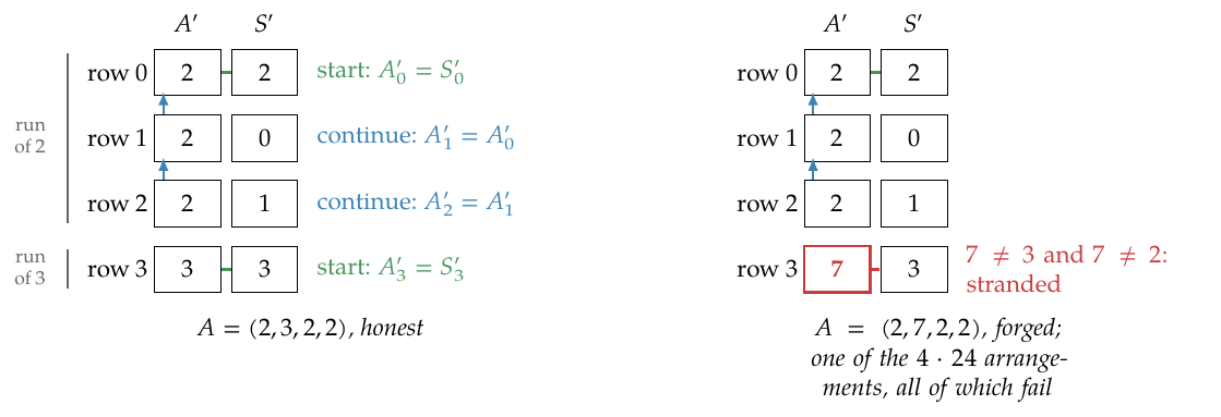
Membership of every entry of a column $A$ in a table column $S$ is, like a copy constraint, a statement about multisets, but it is not a permutation: $A$ may repeat one table entry and omit others. The prover therefore commits to $A^{\prime}$ , a rearrangement of $A$ in which equal values occupy contiguous runs, and to $S^{\prime}$ , a rearrangement of $S$ in which the first row of each run of $A^{\prime}$ holds the matching table value. Two row-local conditions then give membership: each row of $A^{\prime}$ either begins a run, $A^{\prime}_{i}=S^{\prime}_{i}$ , so that its value occurs in $S$ , or continues one, $A^{\prime}_{i}=A^{\prime}_{i-1}$ . The rearrangements are certified by the running product of §2.6 without labels: labelled factors fix one wiring $\sigma$ , whereas here the rearrangements are the prover’s choice, so a single running product with unlabelled factors, row by row $(A^{\prime}_{i}+\beta)(S^{\prime}_{i}+\gamma)$ against $(A_{i}+\beta)(S_{i}+\gamma)$ , certifies that each primed column is a rearrangement of its original. Induction on the row index then gives membership for every row.

Example 2.13 (A two-bit range check on the toy grid).

Constrain cells to two-bit values with the table $S=(0,1,2,3)$ and the column $A=(2,3,2,2)$ . Grouped, $A^{\prime}=(2,2,2,3)$ ; align $S^{\prime}=(2,0,1,3)$ , a rearrangement of $S$ placing $2$ beside the first run and $3$ beside the second. Row $0$ starts a run ( $2=2$ ), rows $1$ and $2$ continue it ( $2$ above), row $3$ starts a run ( $3=3$ ): every check is row-local and every polynomial low-degree, however large the table (Figure 6). The unlabelled product certifies the rearrangements: at the challenges $(\beta,\gamma)=(5,7)$ both $\prod_{i}(A^{\prime}_{i}+\beta)(S^{\prime}_{i}+\gamma)$ and $\prod_{i}(A_{i}+\beta)(S_{i}+\gamma)$ equal $82$ . The forged column $A=(2,7,2,2)$ fails the row checks: its $7$ must start a run in any arrangement $A^{\prime}$ , and no rearrangement of a table without a $7$ can put a $7$ beside it. Over all $4$ arrangements of the forged column and all $24$ rearrangements of the table, the row checks pass for none.

The Action circuit uses lookups of both kinds: it range-constrains each ten-bit word of a decomposition by a lookup into the table $\{0,\dots,2^{10}-1\}$ (the halo2 book’s Decomposition chapter), and it evaluates Sinsemilla by a lookup into a fixed table whose $2^{10}$ rows hold an index $i$ and the two coordinates of the $i$ -th Sinsemilla generator (the halo2 book’s Sinsemilla chapter; the Orchard book’s Circuit chapter records the deployed uses of both). A table fact costs a few committed columns and one more running product, and the gates stay low-degree. The form of the Action circuit’s gates, one gate in full, and its three lookups are given in §4 under “From statement to circuit: arithmetisation in practice”; the exact identities, the boundary row, and multi-column tables come next.

2.8 The lookup argument

Construction 2.14 (Lookup argument).

The objective is that every entry of the column $A(X)$ on the active rows appears as some entry of the column $S(X)$ (the halo2 book’s Lookup argument chapter). The prover supplies polynomials $A^{\prime}(X)$ and $S^{\prime}(X)$ where (i) $A^{\prime}$ is a permutation of $A$ with like values grouped into contiguous runs, and (ii) $S^{\prime}$ is a permutation of $S$ in which the first row of each run of like values in $A^{\prime}$ holds the matching value. The prover commits to $A^{\prime}$ and $S^{\prime}$ ; after receiving challenges $\beta,\gamma$ she commits to a running-product column $Z_{\mathrm{lookup}}(X)$ and proves the four identities, all modulo $Z_{H}(X)$ ,

$\displaystyle\ell_{0}(X)\,\bigl{(}1-Z_{\mathrm{lookup}}(X)\bigr{)}$	$\displaystyle\equiv 0,$	(9)
$\displaystyle Z_{\mathrm{lookup}}(\omega X)\,\bigl{(}A^{\prime}(X)+\beta\bigr{% )}\bigl{(}S^{\prime}(X)+\gamma\bigr{)}-Z_{\mathrm{lookup}}(X)\,\bigl{(}A(X)+% \beta\bigr{)}\bigl{(}S(X)+\gamma\bigr{)}$	$\displaystyle\equiv 0,$
$\displaystyle\ell_{0}(X)\,\bigl{(}A^{\prime}(X)-S^{\prime}(X)\bigr{)}$	$\displaystyle\equiv 0,$
$\displaystyle\bigl{(}A^{\prime}(X)-S^{\prime}(X)\bigr{)}\bigl{(}A^{\prime}(X)-% A^{\prime}(\omega^{-1}X)\bigr{)}$	$\displaystyle\equiv 0,$

the second and fourth additionally masked by the active-row factor of Remark 2.17.

Theorem 2.15 (Soundness of the lookup argument).

Let the columns $A,S,A^{\prime},S^{\prime}$ be fixed before $\beta,\gamma$ are drawn. If the four identities (9) hold on the active rows, with the boundary conditions of Remark 2.17, then except with probability at most $4n/|\mathbb{F}|$ over the challenges $\beta,\gamma$ , every value of $A$ on the active rows equals the value of $S$ at some active row.

Proof.

Let the active rows be $0,\dots,u-1$ (Remark 2.17), and write $A_{i}:=A(\omega^{i})$ , likewise for $S,A^{\prime},S^{\prime}$ , and $Z_{i}:=Z_{\mathrm{lookup}}(\omega^{i})$ . Suppose first that no numerator factor $A_{i}+\beta$ or $S_{i}+\gamma$ with $i<u$ vanishes. The columns are fixed before the challenges, so each of the $u$ values $-A_{i}$ equals $\beta$ with probability $1/|\mathbb{F}|$ , and likewise for $\gamma$ ; by the union bound the supposition fails with probability at most $2u/|\mathbb{F}|$ . Under it, the second identity at row $i<u$ reads $Z_{i+1}\,(A^{\prime}_{i}+\beta)(S^{\prime}_{i}+\gamma)=Z_{i}\,(A_{i}+\beta)(S_% {i}+\gamma)$ , and induction from $Z_{0}=1$ gives $Z_{i+1}\neq 0$ and $(A^{\prime}_{i}+\beta)(S^{\prime}_{i}+\gamma)\neq 0$ for every $i<u$ . Hence $Z_{u}\neq 0$ , the boundary condition forces $Z_{u}=1$ , and multiplying the identities over $i<u$ and cancelling the nonzero $Z_{i}$ gives

\prod_{i<u}\bigl{(}A^{\prime}_{i}+\beta\bigr{)}\bigl{(}S^{\prime}_{i}+\gamma% \bigr{)}=\prod_{i<u}\bigl{(}A_{i}+\beta\bigr{)}\bigl{(}S_{i}+\gamma\bigr{)}.

Set $f(\beta):=\prod_{i}(A^{\prime}_{i}+\beta)$ , $g(\beta):=\prod_{i}(A_{i}+\beta)$ , $f^{\prime}(\gamma):=\prod_{i}(S^{\prime}_{i}+\gamma)$ , $g^{\prime}(\gamma):=\prod_{i}(S_{i}+\gamma)$ and $P:=ff^{\prime}-gg^{\prime}\in\mathbb{F}[\beta,\gamma]$ . If $A^{\prime}$ is a permutation of $A$ and $S^{\prime}$ of $S$ then $f=g$ and $f^{\prime}=g^{\prime}$ , so $P=0$ . If instead, say, $A^{\prime}$ is not a permutation of $A$ , then the multisets of roots $\{-A^{\prime}_{i}\}$ and $\{-A_{i}\}$ differ, so $f\neq g$ by the cancel-and-evaluate argument in the proof of Theorem 2.11 (now over the field $\mathbb{F}$ itself); comparing the coefficients of the top power of $\gamma$ in $ff^{\prime}=gg^{\prime}$ , both $f^{\prime}$ and $g^{\prime}$ being monic of the same degree, would force $f=g$ , so $P\neq 0$ , of degree at most $u$ in each variable, and Lemma 2.9 bounds the probability that the challenges hide the difference by $2u/|\mathbb{F}|$ . The case of $S^{\prime}$ is symmetric. The two terms together are at most $2u/|\mathbb{F}|+2u/|\mathbb{F}|\leq 4n/|\mathbb{F}|$ .

So, with that probability excepted, $A^{\prime}$ is a rearrangement of $A$ and $S^{\prime}$ of $S$ on the active rows. The third identity fixes row $0$ : $A^{\prime}_{0}=S^{\prime}_{0}$ , a table value. The fourth, at every later active row $i$ , says $(A^{\prime}_{i}-S^{\prime}_{i})(A^{\prime}_{i}-A^{\prime}_{i-1})=0$ : either $A^{\prime}_{i}=S^{\prime}_{i}$ , a table value, or $A^{\prime}_{i}=A^{\prime}_{i-1}$ . (At row $0$ the reference $A^{\prime}(\omega^{-1}X)$ wraps around to the last row and carries no information, which is why the third identity is needed there.) By induction on $i$ , every $A^{\prime}_{i}$ equals the entry of $S^{\prime}$ at some active row, hence that of $S$ at some active row; and since every entry of $A$ on the active rows occurs in $A^{\prime}$ there, the claim follows. □

Multi-column tables.

A lookup of $m$ input expressions $A_{0},\dots,A_{m-1}$ against $m$ table columns $S_{0},\dots,S_{m-1}$ is reduced to a single column by a random linear combination with a challenge $\theta$ drawn after the input and table columns are committed:

A_{\mathrm{c}}(X):=\sum_{j=0}^{m-1}\theta^{\,m-1-j}A_{j}(X),\qquad S_{\mathrm{% c}}(X):=\sum_{j=0}^{m-1}\theta^{\,m-1-j}S_{j}(X),

(10)

and Construction 2.14 runs on $A_{\mathrm{c}}$ and $S_{\mathrm{c}}$ .

Proposition 2.16 (Compression of a multi-column lookup).

Let $\theta$ be drawn uniformly after all input and table columns are fixed. If the input tuple at some active row equals the table tuple at no active row, then the compressed input $A_{\mathrm{c}}$ at that row equals $S_{\mathrm{c}}$ at some active row with probability at most $n(m-1)/|\mathbb{F}|$ .

Proof.

For each active table row the difference of the compressed values is a polynomial in $\theta$ of degree at most $m-1$ whose coefficients are the differences of the tuple entries, not all zero; it is therefore nonzero, and the random $\theta$ zeroes it with probability at most $(m-1)/|\mathbb{F}|$ (Math Guide, §“The Schwartz–Zippel lemma”). A union bound over the at most $n$ active rows gives $n(m-1)/|\mathbb{F}|$ . □

Variable tables, where $S$ is itself an advice column, and range checks, where $S$ enumerates the allowed range, are special cases of the same argument.

Remark 2.17 (Active rows and blinding).

The lookup identities, like the permutation identities of §2.6, hold on the active rows only. The deployed system withholds the trailing rows of every column from them: a boundary row and, after it, $n_{\mathrm{blind}}$ blinding rows, which in every witness column (advice, and the permuted and running-product columns of the arguments) hold uniform random values, for the reason “Zero knowledge: hiding the witness in Halo 2” in §4 gives; fixed and instance columns carry no random values. Let $u:=n-n_{\mathrm{blind}}-1$ . Rows $0,\dots,u-1$ are the active rows, row $u$ is the boundary row, and rows $u+1,\dots,n-1$ are the blinding rows. (The letter $u$ indexes a row here; in §3 it denotes a round challenge.) Let $\ell_{\mathrm{blind}}(X)$ be the sum of the Lagrange basis polynomials of the $n_{\mathrm{blind}}$ blinding rows, and let $\ell_{\mathrm{last}}(X):=\ell_{u}(X)$ select the boundary row. Both are computed directly from the domain by both parties; they are not committed circuit columns. Each product-update identity, and the run identity of (9), is multiplied by the factor $\bigl{(}1-(\ell_{\mathrm{last}}(X)+\ell_{\mathrm{blind}}(X))\bigr{)}$ , which is $1$ on the active rows and $0$ elsewhere, so the random rows do not violate the active-row constraints. The wrap-around that closed the loop in Construction 2.10 is gone, so the running product is pinned at the boundary row instead, by $\ell_{\mathrm{last}}(X)\,\bigl{(}Z(X)^{2}-Z(X)\bigr{)}\equiv 0$ , which allows $Z(\omega^{u})\in\{0,1\}$ (the halo2 book’s Lookup argument and Permutation argument chapters). The value $0$ is permitted so that a vanishing numerator factor ( $A_{i}+\beta$ or $S_{i}+\gamma$ ; in the permutation argument $v_{\kappa}+\beta\,\lambda_{\kappa}+\gamma$ ) still leaves the honest prover a satisfying assignment: she sets the product to $0$ from the next row on. The prover cannot force this event, because $\beta,\gamma$ are drawn after her columns are committed. A denominator factor that vanishes at an earlier row than every vanishing numerator factor admits no satisfying running product: the update at that row $j$ reads $0=Z(\omega^{j})$ times a nonzero numerator, and $Z(\omega^{j})\neq 0$ . This happens with probability at most $2u/|\mathbb{F}|$ for a lookup and $N/|\mathbb{F}|$ for the permutation argument, so completeness is overwhelming, not perfect. A boundary value of $0$ is not a certificate of multiset equality, so soundness also excludes the challenges at which a numerator factor vanishes: the bound of Theorem 2.15 includes that term, and Corollary 2.12 adds it for the permutation argument.

2.9 Why the prover cannot wriggle: binding commitments

The random-point argument of §2.4 rests on a hypothesis: Theorem 2.5 assumed the prover’s polynomials were fixed before she saw $z$ . If she could choose $a, b, c, t$ after learning $z$ , she would pick numbers making (5) hold and reveal nothing real. A polynomial commitment enforces that hypothesis.

What a commitment must do.

A commitment to a polynomial $f$ is a short string $C=\mathsf{Commit}(f)$ with two properties, both developed in the Crypto Guide, §“Hiding and binding”:

•

Binding. Having published $C$ , the prover cannot later open it as two different polynomials; $C$ pins down $f$ . Committing first, then receiving $z$ , then opening, leaves her answering for the one polynomial she fixed in advance, the situation Theorem 2.5 assumed.
•

Hiding. The string $C$ reveals nothing about $f$ . This is what will let the proof be zero-knowledge, under “Zero knowledge: hiding the witness in Halo 2” in §4.

A polynomial commitment adds an evaluation proof: given $C$ and a point $z$ , the prover can prove “ $f(z)=v$ ” for the committed $f$ without exposing $f$ , and no prover can produce accepting proofs of two different values at the same point (evaluation binding, Crypto Guide, §“Polynomial commitment schemes”). Theorem 2.5 concerns the idealised protocol, in which the verifier receives the true evaluations of polynomials fixed in advance. Compiled with a polynomial commitment scheme that is evaluation-binding and extractable, the four-step protocol of §2.4 becomes, under compatible composition hypotheses, an argument of knowledge (Crypto Guide, §“SNARKs: succinct non-interactive arguments of knowledge”, Theorem “The compilation recipe, informal”): by its layered extraction, a prover who passes either answers with the true evaluations of polynomials fixed before $z$ , where Theorem 2.5 applies, or breaks the scheme’s evaluation binding or extractability. This volume asserts no bound on the compiled error as a sum of $\deg D/|\mathbb{F}|$ and a commitment term (Remark 4.11, §5). For Halo 2 the extractability of the openings is Theorem 3.5 and, for the deployed opening, Corollary 3.13, under the discrete-logarithm assumption on Vesta, with the generator hash modelled as a random oracle.

How Halo 2 commits.

Encode $f$ of degree $<n$ by its coefficient vector $\mathbf{f}=(f_{0},\dots,f_{n-1})$ ; the running example’s advice polynomial becomes $\mathbf{a}=(90,61,22,24)$ . Let $\mathbb{G}$ be a group of prime order $|\mathbb{F}|$ (deployed: Vesta, of order $p_{\mathsf{Pallas}}$ ), and let $G_{0},\dots,G_{n-1},H\in\mathbb{G}$ be generators derived from a public hash, with $\mathbf{G}:=(G_{0},\dots,G_{n-1})$ ; here $H$ is a group element, not the evaluation domain. The commitment is the single group element

C=\langle\mathbf{f},\,\mathbf{G}\rangle+[r]H=\sum_{i}[f_{i}]\,G_{i}+[r]H,

the Pedersen vector commitment of the coefficient vector with blinder $r\in\mathbb{F}$ (Crypto Guide, §“Pedersen vector commitments”; the mixed inner product of a scalar vector with a vector of group elements is the Math Guide’s, §“The mixed inner product with group elements”). The commitment is perfectly hiding for uniform $r$ and computationally binding under the discrete-logarithm assumption in $\mathbb{G}$ , with the hash modelled as a random oracle into $\mathbb{G}$ (Crypto Guide, §“Pedersen vector commitments”, Theorem “Properties of the vector commitment”): two openings of one $C$ would exhibit a nontrivial discrete-logarithm relation among the $G_{i}$ and $H$ . Proving $f(z)=v$ is proving a statement about an inner product, since

f(z)=\sum_{i}f_{i}\,z^{i}=\langle\mathbf{f},\,(1,z,z^{2},\dots,z^{n-1})\rangle,

and the inner-product argument does this in a logarithmic number of rounds, each halving the vectors, until the claim is trivial: the evaluation proof is $O(\log n)$ group elements, and it needs no trusted setup, because the generators come from a public hash rather than from anyone’s secret (Crypto Guide, §“Polynomial commitment schemes”, the inner-product alternative). Halo 2 uses exactly this one polynomial commitment scheme and no other: the inner-product argument over a group with no pairing (the halo2 book, which the protocol specification names as the definition of the system, § 5.4.10.3, “Halo 2”; its Inner product argument chapter), on the Vesta curve, where the protocol specification places the Action statement’s proofs (protocol specification, § 5.4.9.6, “Pallas and Vesta”). The parameters, the generators and the deployed byte layout are given at the end of §3.

Opening a vector commitment.

For the argument of this section the commitment must bind, so that the prover answers for polynomials fixed before $z$ is drawn. A vector commitment alone does not provide step 3 of the random-point check. The only opening the Pedersen construction offers is the whole vector together with its blinder, $n+1$ field elements: sending it reveals $f$ , and it is no shorter than $f$ . The verifier needs $\langle\mathbf{f},\,(1,z,\dots,z^{n-1})\rangle=v$ established for a committed $\mathbf{f}$ he never sees, in fewer than $n$ group elements. That is the inner-product argument of §3.