1 The provable-security model
This section makes “the scheme is secure” a statement with
mathematical content; every later section states its security
definitions and proofs in these terms. It defines the security
parameter and the adversary, indistinguishability of probability
ensembles, security games and advantage, reductions and their loss, the
standard and random oracle models, and concrete -bit security, and
proves the hierarchy of indistinguishability notions
(Proposition 1.10) and the hybrid lemma
(Lemma 1.13). A security claim is a universally
quantified statement about a precisely delimited class of adversaries;
the groups, fields and curves of the Math Guide carry no
security guarantee by themselves. Unconditional proofs of security are
almost never available, since one would typically imply
1.1 Adversaries and the security parameter
The vocabulary of efficiency is that of the closing section of the Math Guide, recalled here with the refinements cryptography needs.
The security parameter
Schemes are families because security is asymptotic: no scheme with a
fixed finite key length is unbreakable, since an adversary with enough
time enumerates a finite key space. The requirement is that, as
grows, the costs of the honest parties (key generation,
encryption, signing) grow polynomially while the cost of the best
attack grows super-polynomially, ideally exponentially; security is a
statement about the limit
The unary encoding replaces the -bit binary representation of because complexity theory measures running time as a function of input length: in binary, of length , the parameter would allow an algorithm polynomial in its input length only steps—too few to write down a -bit key. The convention is a normalisation only; no substantive result depends on it.
Remark 1.1.
Every quantity in this volume—the adversary’s success probability, its running time, the key length—is a function of , even where the notation suppresses the dependence. A single number—“the advantage is at most ”—either fixes a concrete or describes the function’s behaviour for the of interest.
An algorithm is probabilistic polynomial-time
(PPT) if it is a probabilistic Turing machine—one equipped with a
read-only tape of independent uniformly random bits, its random
tape—and there is a polynomial such that on every input
, and for every setting of the random tape,
halts within steps: the strict, worst-case notion of the
Math Guide (§“Algorithms, running time, and PPT”). We write
Polynomial time. Polynomial time abstracts “feasible computation”: it is closed under composition and invariant across all reasonable deterministic computational models (the strong Church–Turing thesis). The honest parties run in polynomial time so that the scheme is usable; security asserts that no polynomial-time attack succeeds.
Randomness. Honest algorithms need randomness: deterministic encryption leaks whether two ciphertexts encrypt the same message, and key generation must sample secrets unpredictably. The adversary is granted randomness as well, both so that it has the resources of the honest parties and because a deterministic adversary is the special case in which the random tape is ignored.
This volume adopts as standard the non-uniform strengthening that the Math Guide mentions (§“Algorithms, running time, and PPT”).
Definition 1.2 (Non-uniform PPT).
A non-uniform PPT adversary is a family of probabilistic circuits (or, equivalently, Turing machines each supplied with an advice string of length ) such that a single polynomial in bounds the size of . The advice may depend arbitrarily on but not on the particular inputs drawn at run time.
Remark 1.3.
The distinction between uniform adversaries (a single machine that reads and works for all ) and non-uniform ones (a separate circuit per , or a uniform machine with per- advice) is substantive: non-uniformity grants the adversary free precomputed advice tailored to each parameter size, for example a short hint about the group in use for that parameter. Security against non-uniform adversaries is the stronger and now-standard requirement, partly because non-uniform models compose more cleanly under reduction (one may “hard-wire” a fixed good choice of randomness or auxiliary input). All definitions below can be read in either model; hardness assumptions are stated against non-uniform adversaries where the distinction matters, and the choice is otherwise left implicit.
Remark 1.4 (Expected versus strict polynomial time, and quantum adversaries).
Two refinements recur. First, some definitions allow expected polynomial-time adversaries, bounding the average rather than worst-case running time; this matters for certain extraction arguments in zero-knowledge, and is flagged where it arises. Second, for post-quantum security one replaces PPT by quantum polynomial-time (QPT)—polynomial-size circuits of quantum gates followed by a measurement, a model this volume does not formalise; the consequences for the assumptions this volume relies on are taken up under “Quantum adversaries: Shor’s algorithm” in the next section. The structural definitions of this section (advantage, indistinguishability, reduction) are agnostic to which class of adversaries one quantifies over; only the underlying hardness assumptions change.
1.2 Distribution ensembles and indistinguishability
The most basic security goal is that no adversary distinguishes two situations: a real protocol transcript from a simulated one, an encryption of from an encryption of , a pseudorandom string from a truly random one. The situations are formalised as ensembles of probability distributions.
Definition 1.5 (Probability ensemble).
A probability ensemble is a sequence
The statistical distance of the Math Guide (§“Statistical distance”) is recalled for countable supports, which ensembles require; the Math Guide treats finite ones.
Definition 1.6 (Statistical distance).
Let
Proposition 1.7 (Variational characterisation).
For
where the last maximum ranges over all (even computationally
unbounded, deterministic) decision functions
Proof.
The set form is the variational characterisation in the
statistical-distance theorem of the Math Guide
(§“Statistical distance”), whose argument is unchanged over a
countable . Only the reformulation over decision functions is
new: a deterministic is the indicator of the set
Proposition 1.8 (Properties of statistical distance).
The statistical distance is a metric on probability distributions:
Proof.
These are the metric and data-processing parts of the statistical-distance theorem of the Math Guide (§“Statistical distance”), again with the argument unchanged over a countable . □
The grades of indistinguishability below use the asymptotic vocabulary
of the Math Guide (§“Polynomial, exponential, and negligible
functions”). A function
Definition 1.9 (Perfect, statistical, and computational indistinguishability).
Let
-
•
The ensembles and are perfectly indistinguishable, written
, if and are identically distributed for every ; equivalently for all . -
•
The ensembles and are statistically indistinguishable, written
, if their statistical distance is negligible: -
•
The ensembles and are computationally indistinguishable, written
, if for every PPT algorithm (the distinguisher), the function is negligible in . The probabilities are over the draw from the ensemble and over ’s internal randomness.
The three notions form a strict hierarchy, whose second strictness
example needs two primitives, defined here in the form the volume uses
throughout. Write for the uniform distribution on
. A one-way function is a polynomial-time
computable
A pseudorandom generator (PRG) is a polynomial-time computable
Proposition 1.10 (Hierarchy).
For all ensembles
The first implication is strict: there exist ensembles that are statistically but not perfectly indistinguishable. The second is strict provided one-way functions exist: under that assumption there exist ensembles that are computationally but not statistically indistinguishable.
Proof.
If
For strictness of the first implication, let be uniform
on and let be uniform on
For strictness of the second, assume one-way functions exist; then a
PRG exists—the Håstad–Impagliazzo–Levin–Luby theorem,
together with the routine lemma that extends any stretch to the
doubling one, both used without proof—and furnishes an ensemble:
let be a PRG, let
Remark 1.11 (Cost and benefit of computational indistinguishability).
In the strictness example the PRG output and a random string are at statistical distance nearly , because the PRG image is a vanishing fraction of the codomain; an unbounded distinguisher checks membership in the image and succeeds. Computational indistinguishability asserts only that finding an efficient test for membership in that image is infeasible. Information-theoretic security with short keys is impossible; computational security, which rests on conjectured hardness, replaces it and permits both public-key primitives and the encryption of long messages under short keys. Statistical and perfect security, when attainable, are unconditional.
1.3 The hybrid argument
Two lemmas make indistinguishability composable: efficient post-processing cannot create a distinguishing advantage, and a polynomially long chain of pairwise-indistinguishable steps cannot accumulate one. The proof of the first is the simplest instance of a reduction.
Lemma 1.12 (Closure under efficient post-processing).
If
Proof.
Suppose some PPT distinguisher separates
from with advantage
. Define
By
The hybrid argument compares two ensembles connected by a chain of pairwise-close intermediate ensembles. It is the triangle inequality with a refinement that imprecise statements omit: the uniformity hypothesis, which explains why the number of hybrids must be polynomial.
Lemma 1.13 (Hybrid lemma).
Let
are uniformly negligible: a single negligible function
(depending on ) satisfies
Proof.
Fix a PPT distinguisher and let be the uniform bound the hypothesis supplies for . By the triangle inequality applied to the telescoping sum,
and the hypothesis bounds the sum by
Uniformity in is essential, and no argument derives it from the
weaker hypothesis that each is negligible for every
fixed : there the threshold beyond which the -th term
is small can depend on , and the dependence cannot be removed.
For a countermodel, take
Applications usually obtain the conclusion by a stronger, structural
route. Suppose the chain arises from a single underlying
assumption
Remark 1.14.
The hybrid argument is where the restriction to “polynomially many” steps is used. A negligible per-step advantage multiplied by a polynomial number of steps remains negligible; a negligible per-step advantage multiplied by, say, steps need not. Hence constructions that would require exponentially many hybrids yield no security proof.
1.4 Security as a game
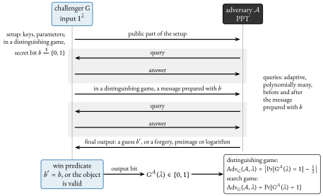
The standard formulation expresses a security definition as a game (or experiment) between a challenger and an adversary : the challenger, following a fixed protocol, sets up the scheme, answers the adversary’s queries, and finally declares the adversary a winner or loser by outputting a single bit.
Definition 1.15 (Security game and advantage).
A security game (or experiment) is a PPT
interactive algorithm, the challenger, that takes ,
interacts with an adversary , and finally outputs a bit
-
•
Distinguishing (indistinguishability) games, where the challenger secretly chooses a uniform bit
and outputs a guess ; the adversary wins iff . Here Trivial guessing achieves winning probability , hence advantage .
-
•
Search (unforgeability/inversion) games, where the adversary must produce a specific kind of object—a forgery, a preimage, a discrete logarithm—and wins iff it succeeds. Here the baseline winning probability is (essentially) , and one sets
Figure 1 draws the interaction.
Definition 1.16 (Security relative to a game).
A scheme is secure with respect to the game if for every PPT adversary ,
The negligible bound may differ from one adversary to another; the claim is universal over the class. The use of on the right makes the definition robust to the polynomial slack that reductions introduce.
Example 1.17 (Pseudorandomness, as a game).
The distinguishing game for a pseudorandom generator
-
1.
The challenger samples
uniformly. If it samples a seed and sends ; if it sends a uniform . -
2.
The adversary outputs a guess ; the game outputs iff
.
The generator is secure iff
Remark 1.18 (Game-hopping).
Game-based proofs are sequences of games: one rewrites the real
security game through a series of games
1.5 Reductions
A reduction is an efficient transformation that converts a successful adversary against a scheme into a successful algorithm against a problem believed to be hard. Its existence proves the implication “ is hard is secure” by establishing the contrapositive “ is broken is solved”.
Definition 1.19 (Computational problem and hardness).
A computational problem consists of a PPT instance generator producing a problem instance together with any side information, and a relation deciding when a candidate output solves the instance. The success probability of an algorithm is
The problem is hard if
Definition 1.20 (Black-box reduction).
Let be a scheme with security game and
a computational problem. A (black-box) reduction from breaking
to solving is a PPT oracle algorithm
with the following per-adversary guarantee: for every
adversary , writing
where is a function fixed by the reduction (not by ) that maps every non-negligible to a non-negligible bound. The running time of is measured with each call to counted as one step, so “PPT” bounds ’s own work, and hence its number of calls to , by a polynomial in ; the running time of is then polynomial whenever ’s is, however many times runs . How far degrades is the reduction’s loss, discussed below. The reduction is black-box because uses only through its input/output interface, making no use of ’s code.
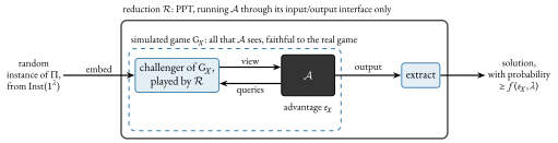
Every reduction has the same structure. To prove “if is hard then is secure”:
-
1.
Assume, towards the contrapositive, a PPT adversary that breaks with non-negligible advantage .
-
2.
Construct a PPT algorithm that, given a random instance of , embeds that instance into a simulated security game for . The simulation must be faithful: the view presents to must follow (perfectly, statistically, or computationally) the distribution of the real game, so that ’s advantage carries over.
-
3.
Run . From whatever does to win its game, extracts a solution to the -instance.
-
4.
Conclude that solves with non-negligible probability, contradicting the hardness of . Therefore no such exists, and is secure.
Figure 2 draws this structure.
Theorem 1.21 (Hard-core security of the Diffie–Hellman-style key, schematically).
Let
Proof.
Suppose is a PPT adversary that, on input a transcript
, outputs with probability
-
1.
The reduction forms the simulated transcript and feeds it to as the public transcript of .
-
2.
Because are uniform in the instance and in the real game, the view of follows identically the distribution of its view in (the simulation is perfect; no loss in faithfulness).
-
3.
When outputs a candidate key , outputs as its answer.
Since the simulated and real views are identically distributed,
outputs
The running time of is that of plus a
constant amount of group bookkeeping, hence polynomial. If
were noticeable, would solve
with noticeable probability, contradicting its
hardness. Therefore is not noticeable, as
claimed. Moreover, since is PPT and is
hard (Definition 1.19, search branch),
This reduction is tight: it calls the adversary once and converts advantage into success probability exactly . Most reductions incur a loss, quantified as follows.
Definition 1.22 (Reduction loss and tightness).
Consider a reduction that transforms an adversary
running in time with advantage into a
-solver running in time
the ratio of the solver’s work-per-success to the adversary’s
work-per-success. A reduction is tight if
Remark 1.23 (Why loss matters concretely).
Asymptotically, loss does not affect the conclusion: a polynomial
loss factor turns a negligible advantage into a negligible advantage
and a hard problem into security. Concretely, however, loss carries a
cost. Suppose a scheme reduces to a problem
believed to offer bits of security, but the reduction loses a factor
Remark 1.24 (Rewinding and the forking lemma, in brief).
A recurrent source of large loss is rewinding: running the
adversary, recording its behaviour, then restarting it from a saved
state with fresh randomness on some branch to obtain a second,
correlated transcript. From two transcripts that share a prefix but
diverge afterwards one can often extract a secret (e.g. two valid
signatures on the same commitment yield the signing key, or two
accepting proof transcripts yield a witness). The forking
lemma, stated as the general forking lemma under “Security in the
random oracle model and the forking lemma”, quantifies the success
probability of obtaining such a pair: if the adversary succeeds with
probability after at most random-oracle queries
whose answers are drawn from a set of size , the forked run
succeeds with probability at least
1.6 The standard model and the random oracle model
The assumptions a proof makes define the model in which it resides. Two models predominate.
Definition 1.25 (Standard model).
A proof resides in the standard model if it assumes only the computational hardness of explicitly stated problems (factoring, discrete logarithm, the decisional Diffie–Hellman problem of the next section, and so on) and grants the adversary no idealised access to any component of the scheme. Every primitive, including every hash function, is a concrete algorithm whose code the adversary may inspect and exploit.
Definition 1.26 (Random oracle model).
A proof resides in the random oracle model (ROM) if it idealises one or more hash functions as a random oracle: a publicly accessible function that, on each distinct input, returns an independent, uniformly random output of the appropriate length, consistently answering repeated queries with the same value. The oracle is available to the honest parties, to the adversary, and, in particular, to the reduction. No party holds the “code” of ; it can only be queried.
Real hash functions are fixed, public algorithms, not truly random functions. The idealisation is adopted because it gives the reduction two capabilities that the standard model withholds and that render many otherwise-intractable proofs tractable.
Remark 1.27 (The powers of the random oracle: observability and programmability).
In the ROM the reduction simulates the oracle for the
adversary. Observability: the reduction sees every query the adversary
makes to . Since the adversary, to use a hash value
meaningfully, must query it, the reduction learns the adversary’s
intermediate computations—for instance the preimage the adversary is
about to hash. Programmability: the reduction may choose each
oracle answer on the fly, subject only to the answers appearing
uniform and consistent. It can therefore plant its hard-problem
instance inside an oracle response—e.g. set
Example 1.28 (The benefit of the ROM: full-domain hash, sketched).
In the “full domain hash” signature, the signer signs a message
as
Remark 1.29 (The status of the ROM: heuristic, not theorem).
A proof in the ROM is a proof about an idealised model: deploying the scheme instantiates with a concrete hash function, and the proof does not formally transfer—a ROM proof rules out all attacks that treat the hash as a black box, while offering no guarantee against attacks on the specific structure of the chosen hash. The case for trusting it runs in three steps: prove the scheme secure against a perfect random oracle; instantiate with a hash believed to have no exploitable structure; and observe that any remaining attack must exploit structure the random oracle lacks, so would be a direct break of the presumed structure-free hash. The gap is nonetheless a theorem: Canetti, Goldreich, and Halevi exhibit contrived schemes provably secure in the ROM yet insecure under every efficiently computable instantiation, so no concrete hash soundly instantiates the oracle for all schemes. No natural deployed scheme is known to be affected; this volume treats a ROM proof as strong positive evidence, not a guarantee, and prefers a standard-model proof when one is available at comparable cost. A quantum adversary (Remark 1.4) queries the oracle in superposition, a single query addressing a weighted combination of all inputs at once; in the resulting quantum random oracle model (QROM) the two powers of Remark 1.27 become subtler and classical ROM theorems do not automatically carry over, so post-quantum claims for arguments made non-interactive by hashing the transcript (the Fiat–Shamir transform, developed under “The Fiat–Shamir transform: from interactive to non-interactive”) must be made in that model.
Remark 1.30 (Relatives: CRS, generic-group, and algebraic-group models).
Further idealisations, between and beyond these two models, are relevant to the proof systems this volume targets. The common reference string (CRS) model posits a trusted public string sampled from a prescribed distribution, used by many succinct proof systems. The generic group model (GGM) idealises the group dual to the manner in which the ROM idealises a hash: the adversary may only perform group operations through an oracle on opaque “handles”, never exploiting the bit representation of group elements; it is the standard setting for lower bounds on discrete-log-type problems. The algebraic group model (AGM) is an intermediate, milder idealisation requiring the adversary to “explain” every group element it outputs as a known combination of its inputs. These models trade realism for provability along the same axis as the ROM; later constructions name the model wherever they require one.
1.7 Concrete security and the bit-security budget
Asymptotic security establishes that a scheme is eventually secure, not whether a deployment with given parameters resists an adversary with a given budget. Concrete (or exact) security settles the latter by explicit bounds on running time and advantage.
Definition 1.31 (Concrete security: -security).
Fix the security parameter to a concrete value (so all sizes are
fixed). A scheme is -secure for a game
if every adversary running in time at most has
advantage
Definition 1.32 (-bit security).
A scheme (or problem) is commonly said to offer bits of security when the cheapest known attack achieving constant success probability (say at least ) costs on the order of elementary operations. A proof may justify the stronger, explicit claim that every adversary running in time has advantage at most about , but that linear advantage bound is not implied merely by the absence of a faster known attack. Thus “-bit security” is a concrete estimate, relative to a specified attack model and state of knowledge, that breaking the scheme costs roughly work.
The security parameter is chosen so that the resulting
concrete scheme delivers the desired number of bits of security. In
the cleanest case the two coincide,
Example 1.33 (Why for discrete logarithm).
For a generic-group or hash-based primitive, doubling the output
length doubles the bit security: a hash with -bit output offers
-bit collision resistance—by the birthday bound (Math
Guide, §“The union bound and a birthday calculation”)—and
-bit preimage resistance, so the parameter and the security
level are proportional. For discrete-logarithm-based primitives the
accounting differs. In a group of prime order
Remark 1.34 (Reading a bit-security budget end to end).
The preceding components combine into a parameter-selection
procedure. First, the target security level is fixed
(commonly ). Second, the underlying hard problem and the cost
of its best attack as a function of the parameter are identified
(e.g. for elliptic-curve discrete log), and the
parameter is set so the problem itself offers bits (here
Remark 1.35 (Scope of a security proof).
A proof of security is a proof relative to a model: a definition of the goal (the game), a class of adversaries (PPT, possibly non-uniform or quantum), and a set of assumptions (the hard problems, and any idealisation such as the ROM). It guarantees nothing outside that model: side-channel leakage (timing, power), faulty randomness, implementation bugs, broken assumptions, and goals the game did not capture all lie beyond its reach. The framework does not render schemes unconditionally safe; it renders the conditions of safety explicit, falsifiable, and modular, so that progress on assumptions and attacks translates into recalibrated guarantees. Every construction in this monograph is analysed within this framework.