4 The Halo 2 proof system
This section defines the Halo 2 proof system as deployed for the Orchard Action statement: the Action circuit, the instance column, the transcript, the multipoint opening, the protocol, and its zero knowledge. It combines the arithmetisation of §2, which reduces a circuit to committed polynomials and identities among them (the gates, the permutation argument for the wiring, the lookup argument for table membership), with the polynomial commitment of §3, which opens a committed polynomial at a point in logarithmically many group elements and is binding under the discrete logarithm on Vesta. The abstractions the Crypto Guide owns, the non-interactive argument and the SNARK, the polynomial interactive oracle proof, the Fiat–Shamir transform and the polynomial-commitment interface, are recalled at the point of use. Halo 2 is a transparent PLONKish argument: the parameters of its commitment scheme are derived by hashing to the curve and carry no trapdoor (§3.8), and for the Orchard Action circuit its polynomial commitment works over Vesta. The protocol specification defines Action proofs as proofs of the Halo 2 proving system described in the halo2 book (protocol specification, § 5.4.10.3, “Halo 2”); this section cites the book, by chapter, as the specification of the protocol, and names an implementation only for a behaviour that neither document fixes.
The subsections treat, in order, the Action circuit as a PLONKish circuit (its gates, one gate in full, its lookup arguments and its column polynomials); the instance column; the Fiat–Shamir transform and the deployed transcript; the multipoint opening argument; the complete protocol in seven phases; its zero knowledge; and the compiled-polynomial-IOP pattern the protocol instantiates. Recursion is not deployed by Orchard and is treated in §7.
Notation.
The constraint degree is , as Definition 2.7 fixed it; the letter is the committed vector length of §3, which equals the row count throughout this section. The letter carries three meanings; two come from the sections this one joins: §2 writes for the evaluation domain and §3 for the blinding generator of the Pedersen commitment. Here the domain appears only through its vanishing polynomial , its Lagrange basis and its rows ; a bare inside a commitment formula is the blinding generator, as in §3. In §4.3 and the security statements the letter also names the transcript hash, modelled as a random oracle, as in the Crypto Guide; there it is applied to arguments, , or called the hash or the oracle. The letter is the evaluation challenge of phase 5; the running example’s witness is written by its value here and in §6.
4.1 From statement to circuit: arithmetisation in practice
Definition 2.7 says what a PLONKish circuit is; the deployed instance is the Orchard Action circuit. The protocol specification fixes the statement it proves, the Action statement (protocol specification, § 4.18.4, “Action Statement (Orchard)”), and requires every Action proof to verify under the verifying key identified by the current Orchard circuit version (protocol specification, § 4.6, “Action Descriptions”, consensus rules). No specification or ZIP fixes the parameters of the circuit behind that key; they are those of its implementation, orchard. As a PLONKish circuit in the sense of Definition 2.7 it has the field , rows, ten advice columns, one instance column and twenty-nine fixed columns, among them its selector columns and the three columns of its lookup table; the constraint-degree bound ; and three lookup arguments into that table, of rows. Its custom gates encode the conditions of the Action statement, using among others complete and incomplete addition on Pallas, the distinction the Math Guide draws in §“Explicit affine formulas” (its remark on complete versus incomplete addition). This subsection gives the form of the gates, one gate in full, the three lookup arguments, and the column polynomials on which every argument of §2 operates.
Key and witness.
The verifying key is a deterministic function of the commitment parameters and the circuit description: the values of the fixed columns, the gates, the lookup arguments and the permutation of Definition 2.7. For the Action circuit it is a fixed consensus parameter, the key the consensus rule above identifies. The prover’s witness is the content of the advice columns. A copy constraint places two cells in one cycle of (Construction 2.10), and the public inputs are bound to advice cells in this way (§4.2).
4.1.1 Custom gates
Every custom gate of the deployed circuit, a gate in the sense of Definition 2.7, has the form
where are columns read at rotations , is a polynomial, and the selector is a polynomial in the fixed columns that is zero on every row where the gate does not apply (the halo2 book’s PLONKish Arithmetization chapter). The gate is required to vanish at every row; on the rows where is zero, the blinding rows among them, it holds whatever the cells contain. The universal gate of vanilla PLONK is the special case of §2.5.
4.1.2 The incomplete-addition gate
The incomplete-addition gate of the Action circuit constrains for affine points and of Pallas with . It has one selector and four equality-enabled advice columns , , and ; it reads at the current row and at the next row of the same two columns , , so that occupies the selector row and the row below it. Its two constraints are
| (31) | ||||
| (32) |
(the halo2 book’s Incomplete and complete addition chapter).
Theorem 4.1 (The gate is the chord formula with the slope eliminated).
Let and be affine points of a short Weierstrass curve with , and set . For a pair the following are equivalent:
- 1.
-
2.
and ;
-
3.
by the chord formulas of the Math Guide (§“Explicit affine formulas”), and .
Proof.
(i)(ii). Since , dividing the first bracket by and the second by are invertible operations: the first bracket vanishes exactly when , and the second exactly when . The gate stores the cleared forms because a constraint must be a polynomial in the cells, and a division is not.
(ii)(iii). The -equations are the same equation rearranged. For the -equations, the chord formula uses the slope of the line through and , which is whichever endpoint is subtracted from which, and the identity gives ; hence , which is (ii)’s -equation with moved across. □
On the -point toy curve of §3.7, over , the chord formulas give for and , and both brackets are at . On Pallas, with and , both brackets are again at the chord sum.
Degrees.
The bracket of (31) has degree three in the cells and that of (32) degree two; with a selector column taking values in the constraints have degrees four and three. The deployed key combines selectors into shared fixed columns (the halo2 book’s Selector combining chapter), which can raise both degrees, keeping them within the deployed bound .
Layout.
The selector is on row , which holds and , each coordinate copy-constrained to the cell it came from; row holds (Table 9). The slope occupies no cell: the identities (31)–(32) verify the sum without it, which is what Theorem 4.1 says. By that theorem the two constraints force , a point of the curve, and because excludes .
| row | |||||
|---|---|---|---|---|---|
| – | – | – |
The excluded inputs.
If , both brackets vanish identically, since every term carries a factor or , and is unconstrained. If , the bracket of (31) reduces to , which is nonzero because Pallas, of prime order, has no point of order two, and no assignment satisfies the gate. The Action circuit applies this gate only to non-identity inputs with : it sums the window multiples of fixed-base scalar multiplication for every window but the last, an offset in the window table excluding the identity and the doubling case there, and adds the last window, whose sum can be the identity or a doubling, with the complete-addition gate (the halo2 book’s Fixed-base scalar multiplication chapter).
4.1.3 Lookup arguments of the Action circuit
A gate asserts only polynomial identities. “This value has ten bits” and “this point is the -th Sinsemilla generator” are set memberships, and §2.7 showed why no low-degree gate on the cell alone states them; the circuit states them as lookup arguments. Each is one instance of Construction 2.14, the input expressions playing and the table columns , compressed by the challenge as in (10) whenever .
The table.
The Action circuit has three lookup arguments, one range check and two Sinsemilla generator lookups, and all three use one table. It holds, for ,
in three table columns , where is the -bit little-endian encoding of the integer , the generator table is defined by the protocol specification (§ 5.4.1.9, “Sinsemilla Hash Function”), and the hash that derives it is the Crypto Guide’s (§“Sinsemilla: an algebraic hash-based commitment”; the hash-to-curve pipeline is §“Hashing to a curve point”). The first two rows are:
| row | coordinates of , hexadecimal |
|---|---|
Unused table rows.
On every active row (Remark 2.17), each of , and holds its row- value, so that every active row of the table is a genuine entry, or . Rows left at would add the tuple , which is no entry, since row is the only entry with index and , and which an input tuple could then match.
The range check.
The range-check lookup is
| (33) |
with and the running-sum advice column at the current and next rotations. With the input is a running-sum step: the prover witnesses on successive rows, so the expression recovers the limb , and membership in asserts that each limb has ten bits. With the cell itself is looked up. Every range check of the Action circuit is either an instance of this lookup, a limb of fewer than ten bits being looked up together with its shift to ten bits, or, for a range of values, the gate ; the three-bit windows of fixed-base scalar multiplication and the single bits use the gate (the halo2 book’s Decomposition chapter).
The Sinsemilla generator lookup.
The Sinsemilla lookup is the three-column instance
| (34) |
where recovers the ten-bit message word from the hash’s own running-sum decomposition of its message, and is an expression in a fixed column that evaluates to on the interior rows of a message piece and to on its final row, where the trailing running sum is implicitly zero. The coordinate is not a cell but a polynomial expression in the queried cells equal to the -coordinate of the generator added (the halo2 book’s Sinsemilla chapter).
Expression-valued inputs.
Lookup inputs may be arbitrary expressions over queried cells, not merely cells. The Sinsemilla lookup asserts that the generator added is with no advice cell holding that generator’s -coordinate. The branches set the input tuple of every row with to table row , so the assertion of Construction 2.14, that every active row’s input tuple appears in the table, holds with nothing to exempt.
4.1.4 Column polynomials and the quotient
Every column, advice, fixed and instance, is a vector of field elements, and its polynomial is its interpolant over the rows, of degree : the column polynomials of §2.5. The trailing rows of each advice column hold uniformly random field elements, the blinding rows of §4.6, on which every selector is zero and which Remark 2.17 exempts from the permutation and lookup arguments.
The quotient.
Each gate polynomial is evaluated with the committed column polynomials substituted for the queried cells, a query at rotation reading , and the resulting polynomials, together with the permutation identities (7) and the lookup identities (9), are folded with powers of a challenge and divided by . The result is the quotient of phase 4 of “The complete Halo 2 protocol” (§4.5), where the folding and the division are written out (the halo2 book’s Vanishing argument chapter).
The running example.
The running example of §2.2 stands at the same point: it interpolated a four-row trace into , the five selector polynomials and , and assembled the one polynomial of degree whose divisibility by , with the quotient of degree , the rest of the protocol certifies.
The deployed parameters.
For the Action circuit , and , the bound holding for its gates and for its permutation and lookup identities. The quotient therefore splits into chunks of degree below , derived in §4.5. The two arguments this construction leans on are the ones §2 proved: the permutation argument of §2.6 stands behind every copy constraint, and the lookup argument of §2.8 behind the lookups (33) and (34).
4.2 Instance columns and binding the public statement
Definition 2.7 lists instance columns beside fixed and advice columns, and the arguments of §2 treat them like any other column. This subsection states how the instance column binds a proof to its public statement.
The public input of the running example.
In the running example the target is public, so it is not advice but instance data: it sits in the public-input polynomial of (2), which the verifier builds himself from the column ; its interpolant of §2.2 takes the value on row and elsewhere. A prover who claimed that has a root would face a different , one with in place of , and her honest trace would no longer vanish on the rows: the fourth gate would read . The public input enters the polynomial whose divisibility Theorem 2.5 tests, and an accepted proof attests the statement for the verifier’s public values.
Definition 4.2 (Instance polynomial).
An instance column is a public-input column: its entries are not part of the witness, and both parties agree on them before verification. Like every other column it is interpolated over the rows in the Lagrange basis,
with and for (§2.5; the Math Guide, §“The Lagrange basis on ”). The public values occupy designated rows, and every other is .
Binding by copy constraints.
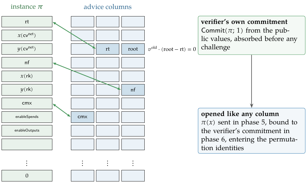
The deployed circuit binds the public values through the permutation argument of §2.6, not through a gate. The instance column is equality-enabled, so it participates in the permutation ; it is one of the fifteen columns counted under “The deployed chunking” there, beside the ten advice and four fixed ones. Each designated instance cell is copy-constrained to an advice cell that the circuit’s constraints read (the halo2 book’s Permutation argument chapter for the mechanism), so a satisfying assignment exists only when those advice cells hold the public values the verifier supplied (Figure 10). The alternative, a dedicated gate with a selector active exactly on the designated rows, is not used: the copy constraint reuses the permutation argument, at no extra gate degree.
The instance commitment.
The verifier does not take from the prover. Both parties compute the commitment to each instance polynomial from the instance values (the halo2 book’s Circuit commitments chapter), with the public blinding factor in place of a random one so that the two computations agree, and absorb it into the transcript before the first challenge is drawn, in phase 1 of §4.5; every Fiat–Shamir challenge thereby depends on the public input. The book fixes the factor for the fixed columns only; for the instance columns it is the choice of the implementation, halo2_proofs. Thereafter the instance column is treated like any other: its claimed evaluation appears among the phase-5 evaluations, enters the permutation identities as one of the of Construction 2.10, and the multipoint opening of phase 6 binds it to the instance commitment. Because the verifier computed that commitment himself, from the instance values he verifies against, the prover has no freedom over : an evaluation inconsistent with the verifier’s own values fails the opening argument, by the evaluation binding recalled in §2.9.
The public input of the Action statement.
The Action statement’s public input is the tuple (protocol specification, § 4.18.4, “Action Statement (Orchard)”): the anchor , the root of the note-commitment tree the spent note is proved against (the Crypto Guide, §“Append-only and incrementally updatable trees”); the net value commitment ; the nullifier ; the randomised verification key ; the extracted commitment of the output note (the Crypto Guide, §“A shielded spend, end to end”); and the flags and , which permit non-zero-valued spends and outputs. The primary-input note of the same section encodes the tuple as the sequence
each integer read as an element of . The Action description specifies the proof with an eighth component, , where permits the output note’s receiver to differ from the input note’s (protocol specification, § 4.6, “Action Descriptions”); from NU6.3 the proof of every Action of either pool is verified with this further public input, which is for every Orchard-pool Action (ZIP 258). Rows to of the instance column hold the nine values above; no normative text fixes the row of the further input, and every other row is (Figure 10). Each is copy-constrained to an advice cell the circuit’s constraints read: , , and to the cells where the circuit computes them; to a cell tied to the computed Merkle root by the gate , which encodes the statement’s condition that or the Merkle path is valid; the two enable flags to cells read by the gates and , which encode, for flags in , the conditions or , and or ; and to a cell read by a gate that, when it is nonzero, equates the coordinates of the receivers of the two notes. That condition is the meaning § 4.6 gives the flag; the list of conditions in § 4.18.4 does not yet include it.
Binding to the instance.
The verifier computes the instance commitment from the public values itself, and the copy constraints tie the designated cells to the advice cells the constraints read; so a witness extracted from an accepting proof satisfies the relation at , not at other public values the prover may target. The probabilistic conclusion, that a prover who knows no witness for , whatever witnesses she holds for other instances, convinces the verifier with at most negligible probability, holds under the knowledge soundness whose status §5 classifies: designed-but-unspecified for the deployed transcript, resting on the discrete logarithm on Vesta or on the algebraic group model, with the transcript hash modelled as a random oracle. Under that hypothesis an Action proof that verifies against an anchor, a nullifier and a value commitment certifies knowledge of a witness consistent with those values.
4.3 Removing the verifier: the Fiat–Shamir transform
The protocols of §§2–3 are public-coin: every verifier message is uniformly random and independent of the prover’s messages, a field element (the point of the random-point check, the pair of the permutation and lookup arguments, the challenges of each opening round) or, in Construction 3.2, the group element ; and the verifier’s decision is a deterministic function of the public input and the transcript. Their soundness requires only that each challenge be drawn after the commitments it tests are fixed.
The transform.
The Fiat–Shamir transform replaces the -th challenge by
the hash of the public statement and of the transcript prefix, the prover’s messages and the earlier challenges, under a fixed hash function (the Crypto Guide, §“The Fiat–Shamir transform: from interactive to non-interactive”). The ordering of §2.9 is enforced because each commitment is an input to the hash that derives the challenge testing it. The toy of §2.4 drew as an interactive challenge; the deployed prover derives every challenge from a hash. The two kinds of challenge are kept apart in what follows: the interactive one is uniform by assumption, the hashed one only in the model in which the hash is a random oracle.
Grinding.
A prover against the compiled argument may vary the inputs of and inspect the resulting challenges. The bound on that freedom uses round-by-round soundness (Canetti, Chen, Holmgren, Lombardi, Rothblum, Rothblum and Wichs, Fiat–Shamir: From Practice to Theory), which Remark 4.11 recalls.
Proposition 4.3 (Fiat–Shamir of a round-by-round sound protocol).
Let be a public-coin interactive protocol whose partial transcripts for a false statement carry a doomed labelling with error : the empty transcript is doomed, a doomed complete transcript is rejected, and from a doomed partial transcript, whatever the prover’s next message, the next challenge leaves it doomed except with probability at most . With modelled as a random oracle, a prover making at most distinct oracle queries, the verifier’s recomputations counted among them, makes the verifier of the Fiat–Shamir transform of accept with probability at most .
Proof.
Each query is a transcript prefix followed by a prover message, and its answer is uniform and independent of everything before the query. The verifier accepts only a transcript that is not doomed, and the empty transcript is doomed, so acceptance requires some query on a doomed prefix whose answer leaves the doomed set; each query does so with probability at most , and the union bound over the at most queries gives . □
The proposition has the form of the halo2 book’s extraction theorem (Protocol Description chapter, “Witness-extended Emulation”, its term ) and of the state-restoration analysis of Ghoshal and Tessaro that §5 cites, where its application to the deployed transcript is classified. For the toy’s identity check, a single challenge with error (§2.4), ten queries exhaust the bound. This volume establishes no round-by-round error for Halo 2, whose binding is computational. At Orchard scale the identity check’s term is about (one Schwartz–Zippel term, in the sense §1.2 fixed), and budgets of , and queries multiply that term alone to , and ; these agree with the of the halo2 book’s algebraic-group-model bound quoted in §5.2, proved for the abstract protocol, whose transfer to the deployed transcript §5 classifies. The permutation argument’s term over , with participating cells (Corollary 2.12), is larger, about .
The hash must take the whole transcript prefix as input: a statement or commitment left out can be chosen after the challenge is seen, the “weak Fiat–Shamir” failure the Crypto Guide records in §“The Fiat–Shamir transform: from interactive to non-interactive”. The bound holds with modelled as a random oracle, a heuristic. The Crypto Guide proves the one-round theorem, with its forking-lemma extractor and its programmed-oracle simulator, and states that a multi-round protocol such as this one needs a multi-round theorem whose hypotheses match the protocol at hand; §5 weighs that theorem against the deployed transcript.
Non-interactivity.
The compiled argument is non-interactive: the proof is one static object, commitments, evaluations and the opening’s scalars, and verification recomputes the challenges by the same hash and runs the same checks. The protocol specification defines a Halo 2 proof as a byte sequence (protocol specification, § 5.4.10.3, “Halo 2”, and its “Encoding of Halo 2 Proofs”), so a full node verifies an Action proof from the transaction alone.
The deployed transcript.
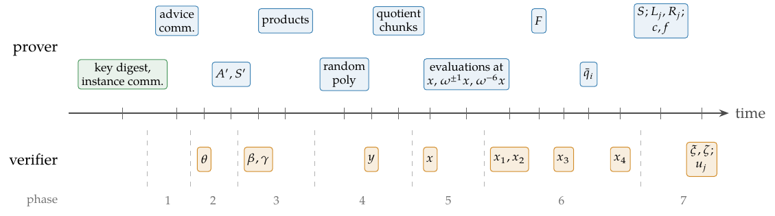
Neither the protocol specification nor the halo2 book fixes the transcript that instantiates the transform; it is that of the implementation, halo2_proofs, and is as follows. The state is a BLAKE2b-512 hash state with the sixteen-byte personalisation Halo2-Transcript (the Crypto Guide, §“Domain separation and personalisation”). Absorbing a point of Vesta appends the bytes ; the identity is not absorbable. Absorbing a scalar appends . Squeezing a challenge appends to the state, which keeps it, and returns the -byte digest of the state read as a little-endian integer and reduced modulo , with no rejection of any value (§3.8). The proof carries each point as its -byte compressed encoding, the -coordinate with the parity of in the top bit (protocol specification, § 5.4.9.6, “Pallas and Vesta”), and each scalar as . Before any prover message both parties absorb, as a scalar, a digest of the verifying key, its BLAKE2b hash reduced into , and then the instance commitments of §4.2, which therefore never appear in the proof. Every prover message is then absorbed in the order the protocol fixes, and each challenge is squeezed at its prescribed point, after everything it must depend on. The proof is the sequence of the prover’s messages in the phase order of Table 10, counted by kind in Table 8; the verifier replays the absorptions and recomputes every challenge. Figure 12 in §4.5 draws the timeline.
4.4 The multipoint opening argument
When the verifier has drawn his evaluation point , the prover has committed to several dozen polynomials and claimed their values at and at rotations of : a running product at and , a permuted lookup input at and , an advice column at every rotation its gates read. Opening each claim with the argument of §3 would cost points per claim, and a one-Action proof makes claims about committed polynomials, the evaluations at and its rotations in Table 8 and the quotient’s ( claims for Actions). Halo 2 reduces all of them to a single opening of a single polynomial at a single point. The reduction combines random linear combinations, division by vanishing polynomials and one random-point check. The letters and below follow the halo2 book’s Multipoint opening argument chapter and are unrelated to the selector polynomials of §2, which are among the polynomials being folded; nor is this the final blinder of the deployed opening (§3.8), which phase 7 sends. The book’s Protocol Description chapter writes the values as , the letter this volume reserves for the round challenges of the inner-product argument; they are written here. The index ranges over sets of query points, not over columns.
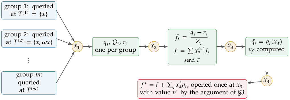
Construction 4.4 (Multipoint opening).
Let be polynomials of degree with commitments under Construction 3.2, each queried at a finite set of points, and let for be the values the prover has claimed. Let be the distinct sets among the and the -th group, enumerated as ; write .
-
1.
Fold each group (). The verifier sends . For each group the prover forms , the verifier forms the same combination of commitments, , which commits to by linearity (Crypto Guide, §“Pedersen vector commitments”), and both form the combined claimed values for . Both interpolate , the unique polynomial of degree with on (the Math Guide, §“Lagrange interpolation”); the verifier can do this from the claimed values alone.
-
2.
Divide out the points (). The verifier sends . The prover forms the quotients , which are polynomials exactly when the combined values equal for every , in particular when every claimed value is true, and combines them into
samples a fresh blinder and sends .
-
3.
A fresh point (). The verifier sends . The prover sends for .
-
4.
The value must take. The verifier computes
the value of if every is a polynomial and every is honest; he can, since and are his to evaluate, and he rejects if some is .
-
5.
One polynomial (). The verifier sends . Both parties form
and run one opening of Construction 3.2 on the statement , the prover’s witness being the coefficient vector of and the blinder , where is the blinder of , the -combination of the blinders of the polynomials in group . The verifier accepts the original claims if and only if that opening accepts.
Two remarks on the shape. Nothing is sent between and , so the deployed transcript squeezes them back to back; they are two challenges because they play two roles, one keeping the polynomials of a group linearly independent and one keeping the quotients of different groups independent. And the reduction is free for the verifier in group operations except for the combinations of commitments, which are a few scalar multiplications per committed polynomial; the one expensive step, the final multi-scalar multiplication, is paid once, inside the single opening. Figure 11 draws the data flow.
Completeness.
If every claimed value is true, then vanishes on and is divisible by (the Math Guide, §“Roots and the factor theorem”), each is a polynomial of degree , so is , and whenever no is ; then holds, and the honest opening of §3 accepts. The verifier’s rejection when is one of the query points, an event of probability at most , is the reduction’s only completeness defect.
Lemma 4.5 (Soundness of the multipoint reduction).
In Construction 4.4, let the committed polynomials and the claimed values be fixed before is drawn, let be a polynomial of degree committed in , fixed before is drawn, let be independent and uniform in , and let . If some claimed value is false, with in group , then the probability that the verifier computes and the polynomial committed in takes the value at is at most
Proof.
The argument takes one Schwartz–Zippel term per challenge (the Math Guide, §“The Schwartz–Zippel lemma”). The fold. The difference is a nonzero polynomial in of degree below , fixed before is drawn, so except with probability the folded claim is false: . The combination. Each is contained in , so each is a polynomial. The polynomial
is fixed once is drawn and is sent, before . At the term and every term with vanish, and
the product over : a polynomial in of degree below , fixed before is drawn, whose coefficient at is nonzero. Except with probability over , then, and is a nonzero polynomial of degree at most . The last fold. Acceptance means , a polynomial equation in of degree at most whose coefficients are fixed before is drawn. Unless every coefficient is zero, that is, unless and for every , a uniform satisfies it with probability at most . The fresh point. If and every , then, since is computed only when , multiplying the first equation by gives , which a uniform achieves for a nonzero with probability at most . A union bound over the four terms gives the stated bound. □
The bound is one more Schwartz–Zippel allowance, of the order of . The opening’s own knowledge error, by Corollary 3.13, lies below it, and that corollary’s witness-or-relation form supplies the binding opening the lemma assumes.
The deployed instance.
In the Action circuit the point sets are five. Every fixed, instance and permuted-label polynomial, the random polynomial of phase 4 and the collapsed quotient are queried at ; the advice columns, five at and five at , according to the rotations their gates read; the permuted lookup input at and the permuted table at ; the lookup running products and the last permutation running product at ; and the first two permutation running products at , the last rotation reaching the boundary row of Remark 2.17 that chains one product into the next. The sets , , , and give the five values , the multipoint evaluations of Table 8, and the whole reduction adds one point and five scalars to the proof.
4.5 The complete Halo 2 protocol
The pieces are now assembled into the Halo 2 protocol (the halo2 book’s Protocol Description chapter, instantiated with the arguments of its Proving system chapters), in seven phases. Throughout, is the constraint field, for Orchard; is the commitment group, the Vesta curve, whose order is (§3.8); the rows are for a primitive -th root of unity , with ; and every commitment is of Construction 3.2, the blinding generator. The protocol has a preprocessed setup and seven phases: (1) advice commitments; (2) lookup compression, challenge ; (3) running products, challenges ; (4) the quotient, challenge ; (5) the evaluation challenge ; (6) the multipoint opening, challenges ; (7) the inner-product opening. Every challenge is squeezed from the transcript of §4.3 at the point named; “the verifier sends” below means that. Table 10 lists the messages with their Orchard counts and Figure 12 draws the timeline.
Setup.
The circuit fixes the columns, gates, lookup arguments and the equality permutation , as §4.1 described; its selectors and lookup tables are fixed columns. Key generation interpolates every fixed column and every permuted-label polynomial of Construction 2.10 and commits to them with the fixed blinding factor (for the fixed columns, the halo2 book’s Circuit commitments chapter); these commitments, with the circuit description, form the verifying key. The transparent parameters of the commitment scheme, the generators , the blinding generator and the inner-product generator hashed to the curve as §3.8 described, together with the domain data, are held separately. All of it is reproducible from public algorithms and the circuit; no secret setup trapdoor exists. Verification is a deterministic function of the parameters, the verifying key, the instance values and the proof.
Phase 1: advice commitments.
Both parties first absorb the digest of the verifying key and the instance commitments of §4.2 into the transcript, so that every subsequent challenge depends on the circuit and on the public input. The prover constructs the advice columns , which with the fixed and instance columns form a satisfying assignment in the sense of Definition 2.7, fills the reserved trailing rows of each with uniformly random field elements, the blinding rows of §4.6, interpolates each to of degree , and sends with fresh blinders . The verifier absorbs the commitments.
Phase 2: lookup compression, challenge .
Phase 3: running products, challenges .
The verifier sends and . The prover commits to the permutation running products, one per chunk of columns as “The deployed chunking” in §2.6 described, and to one lookup running product per lookup, and sends the commitments; the verifier absorbs them. The order is not a convenience. The permuted columns and must be fixed before the challenges that randomise the products are drawn, since Theorem 2.15 bounds the prover’s success probability only over challenges drawn after her columns; a prover who saw first could choose the permutation against them.
Phase 4: the quotient, challenge .
Before is drawn the prover commits to a uniformly random polynomial of degree , sends the commitment, and the verifier absorbs it; its role is the zero-knowledge one explained in §4.6. The verifier then sends . The prover assembles the gate equation, one polynomial
the -weighted combination of the constraint polynomials of the circuit: each constraint of each custom gate with its selector factor, the permutation identities (7) and the chunk-boundary identities, the lookup identities (9), and the boundary identities of Remark 2.17, each masked by its active-row factor where that remark requires. If every constraint holds then every vanishes on the rows, so does, and by (3): the quotient is a polynomial. If some constraint fails at some row, Lemma 4.6 bounds the probability that nonetheless vanishes on the rows, since is drawn after every polynomial in the is committed and after , and .
Lemma 4.6 (Batching by ).
Let be fixed, and let be uniform in . If some does not vanish on the rows, then vanishes on the rows with probability at most .
Proof.
Let . Then is a polynomial in of degree at most with the nonzero coefficient , so it vanishes for at most values of (the Math Guide, §“The Schwartz–Zippel lemma”). □
Theorem 4.7 (Degree of the quotient).
Let every column polynomial and every permuted-label polynomial have degree , and every constraint polynomial degree at most , counting as degree one each column polynomial at a rotation, each , each of , and , and (as in “The deployed chunking” of §2.6). Then
Proof.
A constraint of degree at most is a sum of products of at most such factors, each of degree at most (rotations do not change degrees); so and . Division by , of degree , subtracts . The two forms agree since . □
For the deployed and the bound is , far above the degree bound that the commitment of Construction 3.2 supports with generators, so cannot be committed as one polynomial. The prover therefore uses a fixed proof shape of chunks , each of degree , with
retaining leading zero chunks when the actual degree is smaller, and commits to each chunk separately with its own blinder; there are chunks for Orchard. The count is right because has at most coefficients. Once the evaluation point is drawn, the verifier recombines the chunk commitments, weighted by powers of , into one commitment to the polynomial , whose value at is ; no chunk is ever opened on its own (the halo2 book’s Protocol Description chapter, steps 5 to 8, and note 1 of its “Zero-knowledge and Completeness”).
Phase 5: the evaluation challenge .
The verifier sends . The prover evaluates every committed polynomial the verifier’s identities query, except the quotient chunks, at and at the rotated points the identities reference, for the running products and for any gate reading the next row, for the permuted lookup input and for gates reading the previous row, and , the deployed boundary row, for all but the last permutation product, and sends the claimed values as field elements. The deployed proof also carries the evaluations at of the fixed columns and of the permuted-label polynomials, which the same opening binds to the verifying key’s commitments, and of the random polynomial, bound to its phase-4 commitment. No evaluation of is sent: the verifier computes the expected quotient value from the sent evaluations, evaluating , , and at himself, and enforces it against the collapsed chunk commitment inside the multipoint opening of phases 6 and 7, where the claimed evaluations themselves are bound to their commitments as well. The gate equation is thus checked as the identity , the deployed form of (5).
Phase 6: the multipoint opening, challenges .
The parties run Construction 4.4 on every committed polynomial with a claimed evaluation: the advice columns, the instance column, the fixed and permuted-label polynomials, the permuted lookup columns, the running products, the random polynomial, and the collapsed quotient with its expected value, the last two joining the group. The prover sends the commitment after and the five values after ; after both parties hold the statement .
Phase 7: the inner-product opening.
The parties execute the deployed opening of §3.8, the masked argument in the normalisation of Remark 3.9, on . The prover sends the mask commitment ; the verifier sends and ; then for rounds the prover sends the pair and the verifier answers with ; finally the prover sends the scalars and . The verifier accepts if and only if the deployed equation (29) holds with , and , its one multi-scalar multiplication of length included. Its symmetric counterpart is the masked check (24), which differs from it by the three changes of that remark: the fold normalisation, a change of variables; the factor on ; and the value carried as rather than . Neither it nor (15) is the deployed equation. This is the proof’s end; Table 8 counts its bytes by kind, and nothing else is sent.
Accumulation, not deployed.
In the recursive variant of Halo 2 the verifier is itself a circuit, and that circuit defers the one expensive step of phase 7, the claim of (29), the deployed form (Remark 3.9) of the claim of §3.4, into an accumulator folded with the accumulators of earlier proofs; a single decider at the end verifies all accumulated claims. Orchard does not do this. The protocol specification uses Halo 2 only to prove and verify Action statements and composes no proofs (protocol specification, § 4.1.13, “Zero-Knowledge Proving System”), the Orchard design proposal states that it makes no use of the recursion (ZIP 224), and the verifier pays every deferred multiplication itself; several proofs may share it by the randomised batch check of Lemma 3.14. The variant is developed as the coda of §7.
Costs.
The prover computes one multi-scalar multiplication of length per commitment she sends before the opening, for a bundle of Actions: per Action the ten advice columns, the six permuted lookup columns and the three permutation and three lookup products; shared, the random polynomial, the eight quotient chunks and the multipoint polynomial . She also computes the instance commitments, as the verifier does (§4.2). The opening adds one of length , for its mask commitment , and the cross terms of its rounds, two in each, of lengths in successive rounds. The verifier performs field and group operations for a proof of Actions: he commits to the instance columns (at most ten nonzero values each), recomputes the challenges, evaluates each Action’s gate equation at , combines the commitments of phase 6, and runs the rounds of phase 7; to this he adds the single deferred multi-scalar multiplication of length , which is the linear term that §3.8.1 discussed and that a batch verifier amortises across proofs with fresh random scalars; that batching is distinct from the accumulation above.
| phase | prover sends | verifier squeezes | Orchard count |
|---|---|---|---|
| before | — (both absorb the key digest and the instance commitments) | — | bytes |
| advice commitments | — | points per Action | |
| after , the and commitments, per lookup | points per Action | ||
| after , , the permutation products and the lookup products | , | points per Action | |
| random polynomial commitment; then, after , the quotient chunks | points, shared | ||
| after , the claimed evaluations at and its rotations | scalars per Action; shared | ||
| after , , the commitment ; then, after , the values | , ; ; then | point, scalars, shared | |
| ; then, after , , the pairs for , each followed by ; then , | , ; after each pair | points, scalars, shared |
4.6 Zero knowledge: hiding the witness in Halo 2
Knowledge soundness, classified in §5, concerns what a convincing prover knows; zero knowledge concerns what the proof reveals. Halo 2 is zero-knowledge through two devices, hiding commitments and blinded polynomials, assembled into a simulator. This subsection states what each device achieves on its own, and states the claim for the whole protocol as a cited proposition with its hypotheses.
Evaluations of the running example.
The prover of the running example sends commitments and the evaluations at the random point. An evaluation is a linear equation in the secret coefficients: is one equation in the four unknowns , and evaluations at four distinct points determine the column, hence the secret witness . Halo 2 therefore blinds: the witness trace reserves independent random rows, and every commitment carries an independent random blinding term. Adding random coefficients to a column polynomial would not do: a column polynomial is determined by its row values, and a random coefficient on changes every row, breaking the gates; a random multiple of the Lagrange polynomial of a reserved row changes row alone, which is what a blinding row is. The random values violate no constraint: every selector is zero on the reserved rows, so the gates hold there, and the permutation and lookup identities carry the active-row factor of Remark 2.17. Each column’s openings are then uniform (Lemma 4.8); the joint statement is the proposition of “The simulator” below, whose simulator is one in the sense of the Crypto Guide (§“The simulation paradigm and zero knowledge”).
Hiding commitments.
The commitment of Construction 3.2 is perfectly hiding. The prover commits a polynomial as
with the coefficient vector, the generator vector, and the blinding generator of §3, of no known discrete-logarithm relation to ; the term makes the commitment a uniform group element for every , since generates , so a commitment by itself leaks nothing about what was committed. This is the perfect hiding of the Pedersen commitment, proved in the Crypto Guide (§“The Pedersen commitment” and §“Hiding and binding”) and recalled in §2.9. Every commitment the prover sends in phases 1 to 6, the advice columns, the permuted lookup columns and , the permutation and lookup running products, the random polynomial, the quotient chunks and the multipoint polynomial , has this form with a fresh (the halo2 book’s Protocol Description chapter, which blinds every group element of the protocol, its note 4). The verifying key’s commitments and the instance commitments carry the fixed blinding factor instead: they commit public data both parties recompute (§4.5, §4.2), so there is nothing to hide, and a random blinder would prevent the two computations from agreeing.
Blinding rows.
The prover opens commitments, and an opening reveals evaluations. To keep those evaluations from revealing the witness, the last rows of the table, the blinding rows, carry no circuit data: no gate applies there, and each advice column holds uniformly random field elements on them. By Lemma 4.8 below, a column opened at distinct points outside the rows needs . The halo2 book’s Protocol Description chapter accordingly requires random evaluations of a polynomial opened at rotations of , the extra one covering its opening at the point of the multipoint reduction. In the Action circuit a polynomial is opened at most four times: at three rotations of , for some advice columns and the first two permutation products, and at . The deployed circuit takes , one more than that, a parameter fixed by the implementation, halo2_proofs; with the boundary row of Remark 2.17 its usable rows number . The permutation and lookup running products are blinded the same way, their trailing rows random, and the remark’s active-row factor exempts every one of those rows from every argument, so the random values do not violate a constraint (Figure 13; the halo2 book’s Permutation argument and Lookup argument chapters, their “Zero-knowledge adjustment” sections).
Lemma 4.8 (Openings of a column with blinding rows).
Let be a column polynomial over the rows , let be a set of row indices, the blinding rows, and let be distinct points, none of them a row. With the values on the other rows held fixed, the map from to is affine, and its linear part has rank (Math Guide, §“Bases, dimension, and linear maps”). Consequently, if and the blinding values are uniform and independent, the evaluations are jointly uniform on and independent of the values on the other rows.
Proof.
The map is , a constant plus the linear map with matrix . The Lagrange basis on the rows has the closed form (the Math Guide, §“The Lagrange basis on ”), so with , nonzero on the diagonal because no is a row, , nonzero because is invertible in , and . Hence . Every square submatrix of is nonsingular: take rows and columns with , and suppose coefficients , , not all zero, satisfy for all . Over the common denominator, with of degree ; the polynomial vanishes at the distinct points , so it is the zero polynomial (the Math Guide, §“Roots and the factor theorem”), and then forces for every , since the rows are distinct: a contradiction. Thus has an invertible square submatrix of size , and its rank, at most , equals .
If the linear part is onto , so the affine map is onto, and every fibre is a coset of the same kernel, of the same size . A uniform point of therefore lands in each fibre with the same probability: the image is uniform on . The constant term depends on the other rows but not the distribution, so the evaluations are independent of them. □
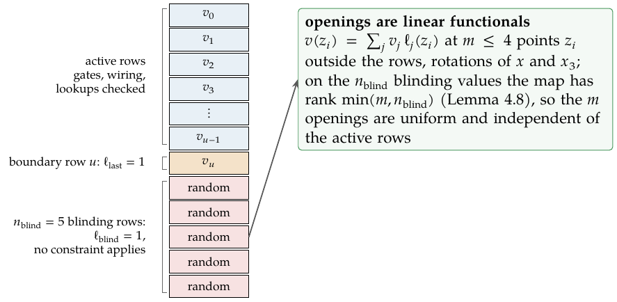
On the toy domain of §2.2, the rank of the lemma’s map was computed for every choice of distinct points among the outside it and for random choices of four: with blinding rows the rank is for one point and for two, and the map is onto; for three points the rank stays and it is not; with the ranks are for one, two and three points, onto each time, and for four points, no longer onto. The threshold is exact: the map is a bijection at and fails first at , so is the condition, and the deployed exceeds the at most openings of any column by one. One hypothesis of the lemma is that the points lie outside the rows: an opening at a row would return a cell, witness or blinder, and the halo2 book’s Protocol Description chapter accordingly excludes challenges in the domain (its note 5). The deployed transcript squeezes full field elements with no rejection, and Corollary 4.10 bounds the effect.
Scope of the lemma.
It is a marginal statement about one column. The proof opens many related polynomials under shared challenges, and the joint distribution of all their evaluations, subject to the public relations among them, the gate equation, the running-product updates, the lookup identities, is not a consequence of the lemma applied column by column. The composition is addressed under “The simulator” below, and its status is stated there.
The quotient and the random polynomial.
The quotient chunks admit no blinding-row treatment: determines them entirely, and the rows of mean nothing. Their commitment blinders, together with the blinding-row randomness they inherit through , protect them instead, and their single collapsed opening at is the publicly computable value , which reveals nothing the verifier did not already hold. There is one more place the quotient could leak: the multipoint reduction evaluates its -group polynomial at the fresh point , and contains the collapsed quotient, whose value at is not a public function of anything. This is why phase 4 commits a uniformly random polynomial before and opens it at alongside the quotient: it joins the same group with the same -weighting, so carries a uniform summand, and the value the prover sends is uniform whatever the quotient’s value at is. The protocol commits that random polynomial for this reason (the halo2 book’s Protocol Description chapter, step 3 and note 2).
Composition.
In each phase the verifier sees only two kinds of object: hiding commitments, which are uniform group elements, and a bounded number of evaluations of the committed polynomials at the transcript’s challenge points. The blinding rows supply randomness which, by Lemma 4.8, makes the openings of each column uniform on its own; a full composition proof must show that this randomness masks the joint evaluations subject to the public relations, and must account for the correlations among advice, products, quotient and multipoint polynomials. The final inner-product opening uses the deployed mask of §3.8, the random polynomial vanishing at whose commitment opens phase 7, in addition to the commitment and round blinders, because Remark 3.7 showed that a final commitment blinder alone would not hide the folded coefficient; the opening of one polynomial was proved statistically honest-verifier zero knowledge there, and that proof is one ingredient of the composition, not the composition.
The simulator.
Zero knowledge requires a simulator for the complete joint transcript, given only the public input. The usual proof samples suitably blinded commitments and evaluations satisfying the verifier’s equations and then programs the random oracle so that the Fiat–Shamir challenges come out as required, in the manner of the Crypto Guide’s one-round simulator (§“The Fiat–Shamir transform: from interactive to non-interactive”). For the interactive protocol the halo2 book exhibits such a simulator and claims the following; this volume records the claim and does not reprove it.
Proposition 4.9 (Zero knowledge of the interactive protocol, cited).
The interactive Halo 2 protocol is perfect special honest-verifier zero knowledge, the simulator being given the verifier’s challenges in advance (the Crypto Guide, §“Sigma-protocols”), for challenge tuples in which every challenge is nonzero and outside the rows and every factor of in (26) is nonzero (the halo2 book’s Protocol Description chapter, “Zero-knowledge and Completeness”). The simulator commits to uniformly random polynomials in place of every polynomial the prover commits in phases 1 to 3 (the book’s : the advice columns, the permuted lookup columns and the running products), the quotient chunks and the multipoint polynomial, and uses its foreknowledge of to choose the mask so that vanishes at .
Corollary 4.10 (Unrestricted challenges).
Let every challenge be uniform in with no value excluded, as the deployed transcript draws them. Then the transcripts of the interactive protocol and of the simulator of Proposition 4.9, run on the same challenges, are within statistical distance , where is the number of challenges, and the values ; for this is .
Proof.
Each challenge has at most excluded values: , the rows, and, for , the value that makes its factor of zero. The challenges have the same distribution in both experiments; on the event that none takes an excluded value the two transcripts are identically distributed by Proposition 4.9, and by a union bound that event fails with probability at most , which therefore bounds the statistical distance. □
Perfect hiding of each commitment and Lemma 4.8 are ingredients of that argument, not by themselves a proof that the joint distribution matches a real execution. For the compiled argument, the Crypto Guide’s compilation recipe (Theorem “The compilation recipe, informal”, §“SNARKs: succinct non-interactive arguments of knowledge”) yields zero knowledge when the polynomial IOP is properly blinded and the corresponding simulation theorem applies; for a multi-round protocol that is a multi-round simulation theorem in the programmable random-oracle model, which this volume neither proves nor cites from a source that proves it for this protocol. Non-interactive zero knowledge of the deployed proof is therefore stated, not proved.
The three properties.
Subject to the hypotheses just named, Halo 2 targets three guarantees for the relation of a PLONKish circuit (Definition 2.7), the three that §1.2 demanded of a proof. Overwhelming completeness: an honest prover holding a satisfying witness convinces the verifier except on negligible transcript degeneracies, a zero inner-product challenge (§3.8, probability per challenge), a point among the query points of the multipoint reduction (“Completeness” in §4.4), an evaluation point on a row, where the verifier’s division by in phase 5 is undefined (probability ), or challenges at which a running-product denominator factor vanishes at an earlier row than any numerator factor does (Remark 2.17; probability at most for the permutation argument on participating cells and per lookup on active rows). Knowledge soundness: an efficient extractor, given rewindable access to any prover the verifier accepts with non-negligible probability, outputs a satisfying witness, so that an accepted proof certifies that one is known. Corollary 3.13 supplies the extractor for the opening layer; §5 lifts it to the non-interactive argument, whose challenges are transcript hashes, and classifies what that lifting establishes. Zero knowledge: a witness-free simulator reproduces the proof, exactly for restricted challenges (Proposition 4.9) and within the distance of Corollary 4.10 for the deployed ones. Knowledge soundness is the property of Action proofs that the Orchard balance and nullifier arguments consume, together with the binding signature (protocol specification, § 4.14, “Balance and Binding Signature (Orchard)”) and the consensus nullifier rules (protocol specification, § 3.9, “Nullifier Sets”); zero knowledge is the property the privacy argument consumes.
4.7 Halo 2 as a compiled polynomial IOP
The protocol of §4.5 factors into two layers: a polynomial interactive oracle proof for the relation, and a polynomial commitment scheme, in the sense of the Crypto Guide (§“Polynomial commitment schemes”), that realises the proof’s oracles. Every phase of the protocol belongs to one of the two layers.
The polynomial IOP, recalled.
The Crypto Guide defines the object (§“SNARKs: succinct non-interactive arguments of knowledge”, under “Polynomial interactive oracle proofs”): a public-coin interactive protocol in which, in place of ordinary messages, the prover in each round sends one or more oracles for polynomials of bounded degree, the verifier answers with uniformly random field elements, and at the end the verifier queries each oracle at a small number of points, receiving the evaluations, and accepts or rejects as a deterministic function of the challenges, the evaluations and the public input. Completeness, soundness and knowledge soundness are those of interactive arguments, with oracle access in place of reading the messages, and the soundness analysis is purely algebraic, resting on the Schwartz–Zippel lemma. The one respect in which a polynomial IOP differs from a vanilla interactive argument is that the verifier never reads a prover message in full: it queries a few evaluations of each oracle. That is what renders the verifier succinct even when the polynomials have large degree; the message length is never read, only as many field elements as there are queries.
The compiler, recalled.
The Crypto Guide’s compilation recipe (the same section) turns a polynomial IOP into a non-interactive argument with a polynomial commitment scheme and a random oracle . Setup runs the commitment scheme’s setup. The prover simulates the IOP, replacing each oracle message by its commitment , derives every verifier challenge from the transcript by the Fiat–Shamir transform of §4.3, and supplies, for each of the IOP’s queries, the claimed evaluation together with an evaluation proof (). The verifier parses the transcript, recomputes the challenges, checks each evaluation proof (), and runs the IOP’s accept-or-reject check on the opened evaluations (Figure 14).
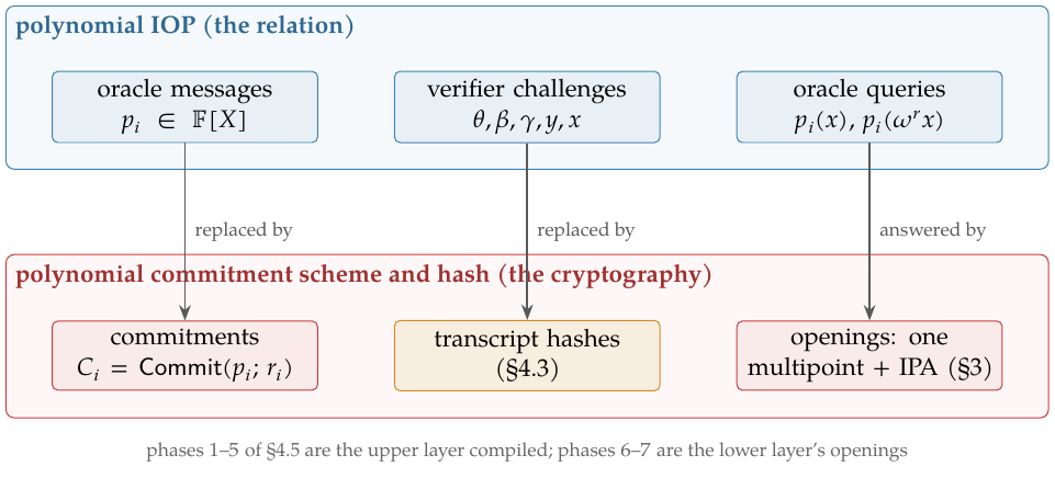
PLONK as a polynomial IOP.
The IOP that Halo 2 compiles is PLONK’s, in the PLONKish generality of §2.5. Its oracles, sent by the prover, are one polynomial per advice column; for each lookup, the two permuted columns and ; the permutation running products, one per chunk, and one lookup running product per lookup; and the quotient , split into chunks below the degree bound. The fixed columns, the selectors among them, and the permuted-label polynomials are preprocessed, part of the verifying key rather than prover messages, which is why they are absent from the list. The verifier’s challenges, in order, are for the lookup compression, and for the permutation and lookup products, for the combination of all constraints into one gate equation, and for the evaluation point. The final check is the gate equation , with the -combination of every gate, permutation and lookup constraint polynomial and the vanishing polynomial of the rows, which the verifier evaluates from the oracles’ values at and at the rotations its constraints read: or for an adjacent row, and , the rotation to the boundary row of Remark 2.17, for the chunk-boundary identities of the permutation argument.
The map onto the phases.
Phases 1 to 5 of §4.5 are this IOP compiled, with one addition: the commitments to the advice, the permuted lookup columns, the running products and the quotient chunks are the oracle messages replaced by commitments, and the random polynomial of phase 4, committed and evaluated at , is the compiler’s addition for zero knowledge (§4.6), not an IOP message; the challenges are the IOP’s challenges squeezed from the transcript, and the claimed evaluations of phase 5 answer the IOP’s oracle queries. Phases 6 and 7 bind those answers to the commitments: the multipoint reduction of §4.4, with its challenges and combined polynomial , followed by the single inner-product opening of . That is the bridge between the abstract compiler and the concrete protocol, and the phase numbering is the one Table 10 uses. Under the hypotheses of the Crypto Guide’s compilation recipe (Theorem “The compilation recipe, informal”) and of Remark 4.11, the compiled protocol has the IOP’s relation and the commitment scheme’s assumptions, transparency, proof size and verifier cost.
Remark 4.11 (The compilation principle, and what it does not say).
Soundness of the compiled argument is not the sum of two numbers, and the notions under which it is proved deserve their names. A polynomial IOP is round-by-round knowledge sound, informally, when its partial transcripts admit a “doomed” labelling that a prover message cannot escape except with bounded probability over the next verifier challenge; a related state-restoration notion lets a prover restore an earlier verifier state and redraw its challenge, which is precisely what a prover attacking a transcript hash can do. Precise equivalence or implication theorems between the two notions require additional conditions on the protocol and on the extractor, and this volume does not identify them. The Crypto Guide’s compilation recipe (Theorem “The compilation recipe, informal”, §“SNARKs: succinct non-interactive arguments of knowledge”) assumes a complete, knowledge-sound public-coin polynomial IOP; a correct, evaluation-binding and extractable commitment scheme; compatible composition hypotheses; and a suitable multi-round Fiat–Shamir theorem in the random-oracle model. For a multi-round protocol such as Halo 2 this volume reads those hypotheses as three: the IOP has a round-by-round or state-restoration knowledge-soundness theorem; the commitment scheme is extractable and evaluation-binding in a form compatible with it; and the transcript satisfies the hypotheses of an appropriate multi-round Fiat–Shamir theorem. The conclusion is that the compiled protocol is a non-interactive argument of knowledge in the random-oracle model, by layered extraction: the commitment scheme’s extractor recovers the committed polynomials, converting the argument’s prover into an IOP prover; the multi-round Fiat–Shamir theorem transfers the round-by-round or state-restoration guarantee to the non-interactive setting; and evaluation binding ensures that the opened evaluations are those of the extracted polynomials. What it does not say is that the knowledge error is determined by two scalars, the IOP’s knowledge error and the commitment scheme’s extraction error, added together: the exact error and the query loss depend on the definitions and on the extraction model, and §5 names the theorems that fix them for the analysed protocol and classifies their instantiation to the deployed transcript.
Delegated results.
The subsection proves nothing afresh. The commitment interface with its hiding, binding and extraction properties is the Crypto Guide’s (§“Polynomial commitment schemes”); the Fiat–Shamir transform and its random-oracle security are the same volume’s (§“The Fiat–Shamir transform: from interactive to non-interactive”); the definitions of completeness, soundness and knowledge soundness for interactive arguments used above are its (§“Interactive proofs, zero knowledge, and SNARKs” and §“Knowledge soundness and extractors”); and the Schwartz–Zippel lemma and the vanishing polynomial of the rows are the Math Guide’s (§“The Schwartz–Zippel lemma” and §“The evaluation domain and its vanishing polynomial”). The volume adds the instantiation: which oracles, which challenges, which openings, and the one commitment scheme that realises them.