4 Commitment schemes
A commitment scheme lets a sender fix a message in a value, the commitment, and later reveal the message to a receiver: once the commitment is delivered, the sender can no longer alter the message (binding), yet the receiver cannot learn it until it is opened (hiding). This section defines commitment schemes, their setup models, and hiding and binding as games in the sense of §1.4; proves that no nontrivial scheme is both perfectly hiding and perfectly binding (Theorem 4.8); and constructs hash-based, Pedersen, Pedersen vector and Sinsemilla commitments, the pairing-based and inner-product polynomial commitments of §4.9, and verifiable secret sharing. The Pedersen and Sinsemilla commitments require only the discrete-logarithm hardness of §2 and the nothing-up-my-sleeve generators of §3, and most later constructions use them. In Orchard, the value commitments checked by binding signatures, the note commitments accumulated in Merkle trees and the witness polynomials of the Halo 2 proof system are all commitments in this sense; polynomial commitments are the cryptographic component of the succinct argument systems of §9, and verifiable secret sharing serves the threshold signatures of a later volume.
4.1 Commit and reveal
The sender computes a commitment to a message and transmits it. Later, at a time fixed by the protocol, the sender opens the commitment by transmitting the message together with the randomness used to compute it, and the receiver checks the revealed message against the commitment. Hiding protects the sender against the receiver between commit and reveal; binding protects the receiver against the sender at reveal time. Without binding a commitment is no evidence of the message; without hiding it keeps nothing secret. The games of §4.3 formalise the two properties.
4.2 Syntax
Definition 4.1 (Commitment scheme).
A commitment scheme Π for a message space M and randomness space R is a triple of algorithms (Setup, Commit, Open) :
-
•
The algorithm Setup (1 λ) is PPT (§1.1) and outputs public parameters p p , which implicitly determine the message space M p p and randomness space R p p and are an implicit input to the remaining algorithms.
-
•
The algorithm Commit (p p, m ; r) , for
m ∈ M p p and r ∈ R p p , is deterministic given r and outputs a commitment c . We write Commit (p p, m) , without an explicit r , for the probabilistic algorithm that samples r ← $ R p p uniformly and returns r alongside c . -
•
The algorithm Open (p p, c, m, r) is deterministic and outputs a bit: 1 (accept) or 0 (reject).
Correctness requires that honestly produced commitments open:
for all p p in the support of Setup (1 λ) , all
| Open (p p, Commit (p p, m ; r), m, r) = 1 . |
The pair (m, r) is called the opening (or
decommitment) of c . Unless stated otherwise, every scheme in
this volume is canonically opening: Open (p p, c, m, r)
recomputes Commit (p p, m ; r) and checks equality with
c . For such a scheme correctness holds automatically, and a valid
opening of c is precisely a pair (m, r) with
Remark 4.2 (The two phases, and a third concern).
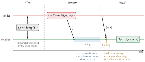
In the commit phase the sender transmits c and nothing else; in the reveal phase it transmits the opening (m, r) and the receiver runs Open . A setup phase producing p p precedes both; who runs Setup , and whether that party can be trusted, is decisive for some of the constructions below (Remark 4.3).
Figure 7 draws the three phases on a time axis, with the threat that each property meets.
Remark 4.3 (Three setup models).
Commitment schemes divide by how much trust their parameters demand.
-
1.
Common reference string (CRS). A trusted party runs Setup and is assumed to erase the randomness behind it. The parameters have internal structure, and knowledge of the discarded randomness—the trapdoor—would break the scheme. Of the schemes treated in this section, only KZG (§4.9) requires this model.
-
2.
Uniform random string (URS), or transparent setup. The parameters consist only of public coins: uniformly random group elements with no known relations among them. There is no trapdoor and no trusted party—anyone can re-derive the parameters from a public seed. This is the regime of the Pedersen and inner-product commitments below. A Pedersen generator derived by hashing to the curve (Construction 3.24) is transparent, although the textbook Setup samples and discards a secret.
-
3.
Plain. No parameters at all, or only a standardised hash function—the home of the hash-based commitment below.
Transparent setup is preferable because a flawed or subverted trusted setup can silently destroy binding, as the KZG trapdoor shows (§4.9).
4.3 Hiding and binding
Both properties are games in the sense of Definition 1.15. In the hiding game the adversary is the receiver; in the binding game it is the sender.
Definition 4.4 (Hiding game and hiding).
Let Π be a commitment scheme and
-
1.
The challenger runs
p p ← Setup (1 λ) . -
2.
The adversary A 1 (p p) outputs two messages
m 0, m 1 ∈ M p p and state s t . -
3.
The challenger samples
r ← $ R p p and computes c = Commit (p p, m b ; r) . -
4.
The adversary A 2 (s t, c) outputs a bit b ′ , which is the output of the experiment.
The hiding advantage of A is
| Adv Π hide (A, λ) := | Pr [Hide Π A (λ, 0) = 1] − Pr [Hide Π A (λ, 1) = 1] | . |
The scheme is computationally hiding if the advantage is negligible (§1.2) for every PPT A ; statistically hiding if it is negligible even for computationally unbounded A ; and perfectly hiding if it is exactly 0 for every adversary and every λ .
Proposition 4.5 (Distributional characterisation of hiding).
A commitment scheme Π is perfectly hiding if and only
if for every p p in the support of Setup and every
pair
| Commit (p p, m 0 ; r) and Commit (p p, m 1 ; r), r ← $ R p p, |
are identically distributed. It is statistically hiding if the statistical distance (Definition 1.6) between them is negligible. (Only the perfect clause is an equivalence: parameters of negligible Setup probability could exhibit large distance without granting any adversary noticeable advantage.)
Proof.
Fix p p and
Definition 4.6 (Binding game and binding).
For a commitment scheme Π and adversary A , the game Bind Π A (λ) runs as follows.
-
1.
The challenger runs
p p ← Setup (1 λ) . -
2.
The adversary A (p p) outputs a commitment c and two openings (m 0, r 0) and (m 1, r 1) .
-
3.
The game outputs 1 iff
m 0 ≠ m 1 and Open (p p, c, m 0, r 0) = Open (p p, c, m 1, r 1) = 1 .
The binding advantage of A is
| Adv Π bind (A, λ) := Pr [Bind Π A (λ) = 1], |
a search game in the sense of Definition 1.15. The scheme is computationally, statistically, or perfectly binding according as the advantage is negligible for every PPT adversary, negligible for every unbounded adversary, or exactly 0 for every adversary and every λ .
For a canonically opening scheme and fixed p p , two openings collide,
that is, win the binding game, precisely when
Remark 4.7 (The asymmetry of the quantifiers).
Hiding quantifies over what can be extracted from a single commitment that the challenger computes and the adversary only observes. Binding quantifies over what can be manufactured: an ambiguous commitment of the adversary’s choosing, under no obligation to follow Commit . The two properties are in tension: the more commitment values a message can take, the better for hiding and the more opportunities for two messages to share one.
4.4 Incompatibility of perfect hiding and perfect binding
Theorem 4.8 (No scheme is perfectly hiding and perfectly binding).
Let Π be a canonically opening commitment scheme with
Proof.
Fix any p p in the support of Setup (1 λ) and
any two distinct messages
| C m := { Commit (p p, m ; r) : r ∈ R p p } |
be the set of attainable commitments to m , and let D m be the
distribution of Commit (p p, m ; r) for uniform r .
Perfect hiding makes D m 0 and D m 1 identical
(Proposition 4.5); identical
distributions have identical supports, so
| Commit (p p, m 0 ; r 0) = c = Commit (p p, m 1 ; r 1), |
and then
Remark 4.9 (The impossibility as a counting fact).
Information-theoretically the theorem counts the bits the commitment
carries. Perfect binding forces the map
Remark 4.10 (Two regimes, two failure modes).
Which property is left computational determines how the scheme fails if its assumption is broken. If binding is only computational, an adversary with enough power—one able to compute discrete logarithms, say—could retroactively change a committed value, and the soundness of any protocol built on top degrades to a computational assumption. If hiding is only computational, such an adversary could retroactively learn a committed value: privacy degrades the same way, and everlasting secrecy is lost once the assumption is broken, even for commitments published long before. Which failure is worse depends on the application: a ledger that publishes its commitments permanently has reason to care about the second, a protocol whose soundness protects funds in circulation about the first.
4.5 Hash-based commitments
The simplest construction hashes the message together with fresh
randomness. It needs two properties from §3: a hash
function
Construction 4.11 (Hash commitment).
Let
| Commit (m ; r) := H (enc (m, r)), |
opened canonically. There are no nontrivial public parameters beyond the choice of H —the scheme lives in the plain model of Remark 4.3.
Proposition 4.12 (Binding of the hash commitment).
If H is collision resistant, the hash commitment is computationally binding.
Proof.
Suppose A wins the binding game: it outputs c with
valid openings (m 0, r 0) , (m 1, r 1) and
Proposition 4.13 (Hiding of the hash commitment, in the ROM).
Model H as a random oracle (Definition 3.13). For
messages of length poly (λ) and randomness length
Proof.
The challenge commitment is
Remark 4.14 (Why the randomness is essential).
The deterministic commitment
Remark 4.15 (Strength profile).
The hash commitment is transparent: it has no parameters and no algebraic structure that a subverted setup could exploit. It is plausibly post-quantum: generic quantum collision finding takes Θ (2 n / 3) queries against an n -bit hash (Remark 2.31), so increasing the output length compensates for the loss. Its weakness is opacity: the commitment is an unstructured bit string, so no algebraic relation on commitments reflects any relation on the committed values; the sum of two hash commitments is not a commitment to the sum of the messages. The Pedersen construction removes this defect at the price of resting on discrete log.
4.6 The Pedersen commitment
The Pedersen commitment works in a prime-order group rather than on bit
strings. Let G be a cyclic group of prime order q , written
additively: for a point
Construction 4.16 (Pedersen commitment).
The algorithm Setup (1 λ) runs
| Commit (p p, m ; r) := [m] G + [r] H, |
opened canonically.
The parameters are two generators G and H whose relative
discrete logarithm
Theorem 4.17 (Perfect hiding).
The Pedersen commitment is perfectly hiding.
Proof.
Fix any attainable
Theorem 4.18 (Computational binding under DLog).
If the DLog assumption holds for G , the Pedersen
commitment is computationally binding. Concretely, from any adversary
A that wins the binding game with probability
ε one constructs B computing discrete
logarithms with probability
Proof.
The algebraic relation comes first. A double opening gives
| [m 0 − m 1] G = [r 1 − r 0] H . |
The case
| s = log G H = (m 0 − m 1) (r 1 − r 0) − 1 mod q . |
A double opening therefore determines the discrete log of H .
The reduction is as follows. On a DLog challenge (G, q, G, Q) , the
algorithm B sets
| Adv dlog (B) = (1 − 1 q) Adv Π bind (A) ≥ ε − 1 q, |
and B ’s overhead over A is a constant number of field operations. □
Remark 4.19 (Equivocation with the trapdoor).
Any party who knows
| r ′ := r + (m − m ′) s − 1 mod q ; |
then
Theorem 4.20 (Additive homomorphism).
For all
| Commit (m 0 ; r 0) + Commit (m 1 ; r 1) = Commit (m 0 + m 1 ; r 0 + r 1), |
and more generally, for all scalars
| [α] Commit (m 0 ; r 0) + [β] Commit (m 1 ; r 1) = Commit (α m 0 + β m 1 ; α r 0 + β r 1) . |
Proof.
Expand and regroup, using commutativity of + in G , the
identity
| [α] ([m 0] G + [r 0] H) + [β] ([m 1] G + [r 1] H) | = [α m 0] G + [β m 1] G + [α r 0] H + [β r 1] H | ||
| = [α m 0 + β m 1] G + [α r 0 + β r 1] H . ∎ |
Remark 4.21 (Value balancing: the homomorphism deployed).
Zcash uses the homomorphism for value balancing. Each transaction value
v i is committed as
Example 4.22 (Value balance and a wrap-around counterfeit in a group of order 1019 ).
We run the balance check of Remark 4.21 in a
group small enough to follow by hand. Take the primes
| C (v ; r) := g v h r mod p . |
No discrete logarithm in G is hard: trying the q exponents in
turn gives
A transaction spends a note of value
| note | value v i | trapdoor r i | C i = C (v i ; r i) |
|---|---|---|---|
| spent | 200 | 731 | 566 |
| created | 150 | 286 | 451 |
| created | 45 | 517 | 139 |
Cancellation. The verifier divides the spent commitment by the
created ones and by the balance under g ,
| C 1 (C 2 C 3) − 1 g − b = 1441 = h 947, 947 ≡ r 1 − r 2 − r 3 = − 72 (mod q) . |
The exponents of g cancel,
Wrap-around. Since
Range. Requiring each of
Prime order. Both theorems above use that q is prime: the
hiding proof of Theorem 4.17 needs
4.7 Pedersen vector commitments
A single group element can commit to a vector of scalars rather than a single scalar.
Construction 4.23 (Pedersen vector commitment).
On input 1 λ and a length
| Commit (p p, m ; r) := ∑ i = 1 n [m i] G i + [r] H = ⟨ m, G ⟩ + [r] H, |
where
Theorem 4.24 (Properties of the vector commitment).
The Pedersen vector commitment is perfectly hiding, and computationally binding under the DLog assumption in G .
Proof.
Hiding. Exactly as in Theorem 4.17: for uniform r the blinding term [r] H is uniform on G , so the commitment is uniform on G regardless of the message vector.
Binding. A double opening with
| ∑ i = 1 n [m i − m i ′] G i + [r − r ′] H = O |
with not all coefficients zero. The reduction B must
extract a single logarithm from a relation among
| G i := [u i] G + [w i] Q, H := [u H] G + [w H] Q, |
and resamples any pair whose generator lands on O . Each
result is uniform on
| c 0 + c 1 s ≡ 0 (mod q), c 0 = ∑ i a i u i + a H u H, c 1 = ∑ i a i w i + a H w H . |
Since the coefficient vector is nonzero and the w -coordinates
are uniform and independent of it, c 1 is uniform on F q ,
hence nonzero with probability
Remark 4.25 (Compression and the cardinality trade-off).
The vector commitment is compressing: n field elements (plus the randomness) map to a single group element, exponentially shorter than the message for large n . Compression is incompatible with statistical binding for a counting reason: there are q n message vectors and only q commitment values, so many colliding openings exist. Binding is therefore only computational—an unbounded adversary finds a colliding opening by solving the underlying discrete-log relation—and the trade-off of Theorem 4.8 appears at the level of cardinalities: a compressing commitment cannot determine its message, so perfect hiding costs it nothing further.
Remark 4.26 (Linearity of the vector commitment).
The vector commitment remains additively homomorphic in both message
and randomness, componentwise:
4.8 Sinsemilla: an algebraic hash-based commitment
Between the opaque hash commitment of §4.5 and the linear Pedersen commitment lie the algebraic hash functions: collision-resistant hashes whose internal operations are elliptic-curve group operations. A zero-knowledge circuit verifying a hash pays for every internal operation, and curve additions in the field over which the proof system works are cheap, while collision resistance still reduces to the discrete logarithm. Sinsemilla, deployed in Zcash Orchard, is a Pedersen-style hash of this kind over a sequence of message chunks, constructed below from the Pedersen hash.
Construction 4.27 (Pedersen hash).
Split the message M into k chunks
| PedersenHash (M) := ∑ j = 1 k [m j] P j ∈ G . |
This is the unblinded Pedersen vector commitment map used as a hash. The output is a group element; composing with a fixed encoding of group elements as bit strings yields an ordinary hash.
Proposition 4.28 (Collision resistance of the Pedersen hash).
Suppose no efficient algorithm finds a nontrivial relation
Proof.
A collision
The Pedersen hash needs one independent generator per chunk, so its generator table grows linearly with the maximum message length. Sinsemilla iterates a two-operand step over a small fixed generator table shared by all chunk positions, and keeps the discrete-log collision reduction.
Construction 4.29 (Sinsemilla hash).
Split the message M into pieces
| S (v) := GroupHash ("z.cash:SinsemillaS", LE 32 (v)), v ∈ { 0, 1 } w, |
with 2 w entries shared by every instance, and the base point is personalised (§3.5) to the enclosing use—a byte string D naming it, such as a note-commitment or Merkle-hash domain—by taking that string as the message:
| Q := GroupHash ("z.cash:SinsemillaQ", D) . |
Both derivations are nothing-up-my-sleeve
(Construction 3.24), so no party knows any
discrete-log relation among
| Acc 0 := Q, Acc j := Acc j − 1 + (Acc j − 1 + S (m j)) = [2] Acc j − 1 + S (m j), |
and outputs the point
| SinsemillaHashToPoint (M) = ∑ j = 1 k [2 k − j] S (m j) + [2 k] Q : |
the integer coefficients are powers of two determined by position alone, and the message enters only through which generator S (m j) each piece selects.
Proposition 4.30 (Collision resistance of Sinsemilla).
Model the table entries S (v) and the base point Q as
independent uniform generators (the nothing-up-my-sleeve
hash-to-curve derivation covers Q as well as the table). Then
any collision in SinsemillaHashToPoint , on inputs for
which its incomplete additions are defined, yields a nontrivial
discrete-log relation among
Proof sketch.
Let
| ∑ j = 1 k [2 k − j] (S (m j) − S (m j ′)) = O . |
Regroup over the distinct table generators: for each value
| c v = ∑ j : m j = v 2 k − j − ∑ j : m j ′ = v 2 k − j, |
and the relation reads
If instead the piece counts differ, say
It remains to treat the exceptional cases. An incomplete addition is
undefined only when its operands are equal or are mutual negatives, so
an input reaching one presents a coincidence
The deployed hash differs from the point hash in two ways. First, the deployed SinsemillaHash applies the Pallas coordinate extractor to SinsemillaHashToPoint (M) , returning its x -coordinate. Collision resistance survives the extraction: equal x -coordinates mean the two points are equal or negatives of one another, and either signed equality yields the same kind of nontrivial generator relation as in the proof above. Second, the message bits are zero-padded to a multiple of the piece width before chunking, so two bit strings of different lengths within the same final piece present identical piece sequences, and the deployed hash claims collision resistance only between inputs of a fixed length for a given personalisation, exactly as the protocol specification § 5.4.1.9 requires (“between inputs of fixed length, for a given personalization input”). Each personalisation domain hashes inputs of a single length, as the Merkle-tree hash MerkleCRH of §10 illustrates. The variable-length argument in the proof above applies to the piece-aligned point presentation, where the piece sequence is the message.
The commitment is obtained from the hash by adding the Pedersen blinding term unchanged.
Construction 4.31 (SinsemillaCommit).
Fix one further independent generator H ′ , hashed to the curve
with its own domain string, so that no discrete-log relation between
H ′ and
| SinsemillaCommit (m ; r) := SinsemillaHashToPoint (m) + [r] H ′ . |
Hiding is inherited unchanged from Pedersen: by the argument of Theorem 4.17, [r] H ′ is uniform on G for uniform r , so the commitment distribution is independent of m , and the scheme is perfectly hiding. Binding rests on discrete log: two valid openings to distinct messages yield either a SinsemillaHashToPoint collision—excluded by Proposition 4.30—or a nontrivial discrete-log relation between H ′ and the hash generators.
Orchard’s note commitment NoteCommit instantiates this map (protocol specification § 5.4.8.4). Its key commitment CommitIvk composes the same map with x -coordinate extraction—the specification’s SinsemillaShortCommit —and returns a base-field element.
Remark 4.32 (In-circuit cost of Sinsemilla).
Outside a circuit ordinary hashes are faster than Sinsemilla; its advantage is verification cost inside one. In a SNARK (§9) the prover re-expresses every computational step as polynomial constraints; a bit-oriented hash such as SHA-256, built from Boolean operations and modular additions foreign to the proof field, costs tens of thousands of constraints per evaluation, whereas Sinsemilla’s per-piece cost is a handful of curve operations in the field over which the proof system works. Orchard uses it for note commitments and Merkle trees: it is cheap to prove and rests on the same discrete-log hardness as the rest of the protocol. A later volume treats the concrete Orchard instantiation: its per-use personalisation strings and the in-circuit handling of incomplete addition.
4.9 Polynomial commitment schemes
A polynomial commitment scheme commits to a polynomial and supports proofs of statements about its values; the succinct argument systems of §9 are built on it.
Definition 4.33 (Polynomial commitment scheme).
Fix a field F and a degree bound d . A polynomial commitment scheme (PCS) is a tuple (Setup, Commit, Open, Eval, Verify) :
-
•
The algorithm Setup (1 λ, d) outputs public parameters p p supporting degree at most d ;
-
•
the algorithm Commit (p p, f ; r) outputs a commitment C to a polynomial
f ∈ F [X] ≤ d , optionally with hiding randomness r ; -
•
the algorithm Open (p p, C, f, r) outputs a bit, verifying that C commits to the whole polynomial f ;
-
•
the algorithm Eval (p p, f, r, z) , for an evaluation point
z ∈ F , outputs a claimed value y = f (z) together with an evaluation proof π ; -
•
the algorithm Verify (p p, C, z, y, π) outputs a bit, checking the evaluation proof against the commitment.
Beyond the hiding and binding of the underlying commitment
(Definitions 4.4
and 4.6), a PCS must satisfy
evaluation binding: no PPT prover can produce a commitment
C , a point z , and two accepting proofs for distinct claimed
values
Remark 4.34 (Rigidity, and why evaluation binding is separate).
A single short commitment can support queries at arbitrary points because polynomials are rigid: a nonzero polynomial of degree at most d has at most d roots (Math Guide, §“The Schwartz–Zippel lemma”), so two distinct polynomials of degree at most d agree on at most d points. A prover that answers a different value at even a single point behaves as one holding a different polynomial. However, an accepting evaluation proof is not an opening of C , so evaluation binding does not follow from the binding of Commit ; each construction below proves it from its own assumption—a strong Diffie–Hellman assumption for KZG, discrete log via a folding extractor for the inner-product scheme. The design problem of a PCS is to make the evaluation proof π short and fast to verify; committing to the coefficient list with an arbitrary commitment scheme does not solve it.
KZG: evaluation in the exponent
The pairing-based scheme of Kate, Zaverucha, and Goldberg achieves constant-size proofs by encoding a secret evaluation point in the parameters.
Construction 4.35 (KZG commitment).
Let
| p p = ([τ 0] G, [τ 1] G, ..., [τ d] G, G ^, [τ] G ^), |
and discards τ . The commitment to
| Commit (p p, f) := ∑ i = 0 d [a i] ([τ i] G) = [f (τ)] G, |
computable from p p by anyone, without knowledge of τ .
Construction 4.36 (KZG evaluation proof).
To prove
| q (X) := f (X) − y X − z ∈ F [X] ≤ d − 1 |
is a genuine polynomial precisely because
| e (C − [y] G, G ^) = ? e (π, [τ] G ^ − [z] G ^), |
which, by bilinearity, is exactly the in-the-exponent form of the
polynomial identity
Proposition 4.37 (KZG evaluation binding, sketched).
Evaluation binding of KZG rests on the d -strong Diffie–Hellman assumption in the bilinear group: given the powers [τ i] G , it is infeasible to produce [(τ − z) − 1] G for any z of one’s choosing.
Proof idea.
Two accepting proofs
| [(τ − z) − 1] G = [(y ′ − y) − 1] (π − π ′), |
exactly the element the assumption declares infeasible. □
Remark 4.38 (Costs and benefits of KZG).
The KZG scheme provides commitments and evaluation proofs of
constant size (one group element each) and constant
verification time (two pairings), all independent of the degree d .
Its setup is trusted: the secret τ is a global trapdoor. Anyone
who learns τ can forge accepting evaluation proofs for
false statements—for any commitment C , any point z ,
and any desired value y , the element
The inner-product alternative
The transparent alternative commits to the coefficient vector with the Pedersen vector commitment and replaces the pairing check by a recursive argument.
Construction 4.39 (IPA-style polynomial commitment).
Let
| Commit (p p, f ; r) := ∑ i = 0 d [a i] G i + [r] H = ⟨ a, G ⟩ + [r] H . |
The construction uses no pairings and no trusted setup.
Evaluation is an inner product: writing
| f (z) = ∑ i = 0 d a i z i = ⟨ a, z ⟩, |
so proving an evaluation reduces to proving an inner-product
relation about a committed vector against a public vector. The
inner-product argument (IPA) proves it recursively: each
round folds the two halves of the coefficient vector—and of the
generator vector—into vectors of half the dimension by taking a
random linear combination dictated by a verifier challenge, sending
two group elements per round (the cross-term commitments L j and
R j ) to account for the mixed terms; after
Proposition 4.40 (Properties of the IPA-based PCS).
The inner-product polynomial commitment has: transparent setup (public-coin parameters, no trapdoor); evaluation proofs of O (log d) group elements; and O (d) -group-operation verification, batchable across proofs. Its binding and evaluation binding reduce to the discrete logarithm assumption in G .
Proof idea.
Binding of the commitment itself is
Theorem 4.24. For evaluation binding
and extractability, one shows the folding protocol is tree
special-sound: from a suitable tree of accepting transcripts,
branching over the verifier’s challenge at each round, an extractor
works back up the recursion and computes a coefficient vector
a consistent with the commitment and the claimed inner
product—a notion this sketch uses only informally and
§9 defines precisely. Two distinct extracted
openings of the same commitment would yield a nontrivial
discrete-log relation among
Remark 4.41 (KZG versus IPA, and the Halo lineage).
KZG gives constant proof size and constant verification, at the price of a structured trusted setup and pairing-friendly curves; the IPA gives transparent setup over a plain curve and rests on nothing beyond discrete log, at the price of logarithmic proofs and linear-time verification. The Halo 2 proof system deployed in Zcash Orchard builds on the inner-product family to avoid trusted setup, and recovers practical verification cost through batching: the deployed verifier folds the final multiscalar multiplications of many proofs into one shared multiexponentiation—each proof’s deferred check is scaled by a fresh random factor and accumulated, and a single combined check is evaluated once. This amortises group operations across a batch, though per-proof verifier work remains linear in d . The Halo lineage’s accumulation technique extends the same deferral across recursively composed proofs, one proof attesting to another’s deferred check—the capability the Pasta cycle of Remark 2.26 was designed to serve—but deployed Zcash does not use recursion: each Orchard proof is verified (in batch) directly.
Remark 4.42 (Hiding variants).
As stated, the KZG commitment is binding but not hiding: it is a deterministic function of f , so committing twice to the same polynomial is visible, and a low-entropy polynomial can be found by search—the failure of Remark 4.14. That is acceptable when the polynomial encodes only public data. When it encodes secrets, as the witness polynomials of a zero-knowledge proof do, randomness is required: KZG is augmented with a blinding summand [r] [γ] G using an extra setup element [γ] G , while the IPA commitment of Construction 4.39 already carries its [r] H and is perfectly hiding by Theorem 4.24. The resulting regime is the perfect-hiding/computational-binding profile of Pedersen (Theorems 4.17 and 4.18), lifted from field elements to polynomials.
From commitments to arguments
A polynomial commitment scheme turns an information-theoretic proof object—a polynomial identity holding over a large field—into a succinct cryptographic argument. The prover commits to its witness polynomials, the verifier challenges at random points, and evaluation proofs show that the committed polynomials satisfy the required identities without revealing them. Soundness comes from Schwartz–Zippel (Math Guide, §“The Schwartz–Zippel lemma”): a nonzero polynomial of low degree is almost surely nonzero at a random point, so an identity that holds at the challenge almost surely holds identically. Binding and succinctness come from the commitment: the prover is bound to its polynomials before seeing the challenge, and the verifier handles only short commitments and proofs. The full compilation, and the precise meaning of “argument of knowledge”, are the subject of §9.
4.10 Secret sharing
Verifiable secret sharing is constructed here because the threshold
signatures of a later volume depend on it and no earlier volume
provides it. The setting is a prime field F q —in the sequel the
scalar field of the
group G of §4.6—and the tool is
Lagrange interpolation (Math Guide, §“Lagrange
interpolation”): a polynomial of degree at most
Construction 4.43 (Shamir t -of- n secret sharing).
Fix a threshold t and a party count n with
| f (X) := s + a 1 X + a 2 X 2 + ⋯ + a t − 1 X t − 1 ∈ F q [X], f (0) = s, |
a polynomial of degree at most
| s = f (0) = ∑ i ∈ I λ I, i s i, λ I, i := ∏ j ∈ I, j ≠ i j j − i, |
where
Correctness of reconstruction is the interpolation theorem: the t
points (i, s i) i ∈ I determine a unique polynomial of degree
at most
Theorem 4.44 (Perfect secrecy below the threshold).
Let I be any set of at most
Proof.
It suffices to treat
| Σ s : F q t − 1 → F q t − 1, (a 1, ..., a t − 1) ↦ (f (i)) i ∈ I, |
from the dealer’s coefficient vector to the coalition’s shares. It
is injective: two coefficient vectors with the same shares give two
polynomials of degree at most
The theorem is the perfect hiding of a commitment, in the form of
Proposition 4.5. Shamir sharing is
not binding: a dishonest dealer can distribute values that lie on no
common polynomial of degree at most
Construction 4.45 (Feldman verifiable secret sharing).
Let (G, q, G) be as in §4.6, so
that F q is the scalar field of G . The dealer shares s
as in Construction 4.43, with
| Φ k := [a k] G ∈ G, k = 0, ..., t − 1, |
the coefficients in the exponent. Party i , on receiving its private share s i , accepts it iff
| [s i] G = ? ∑ k = 0 t − 1 [i k] Φ k . |
An honest share passes: since
Proposition 4.46 (What the Feldman check certifies).
Because G generates the prime-order group G , the map
Proof.
Both claims are injectivity of
The vector (Φ k) k is a
perfectly binding commitment to the polynomial f —the
coefficient list committed entry by entry under the bijection
Remark 4.47 (Leakage of Feldman sharing).
Feldman sharing publishes