Halo 2 Guide The Halo 2 proof system, from arithmetisation to recursion 2 Arithmetisation: from a computation to committed polynomials 4 The Halo 2 proof system

3 The inner-product polynomial commitment

This section constructs the inner-product polynomial commitment that opens the commitments of §2.9 at the verifier’s point. It states the problem, performs one halving step, recurses it into the full argument with both parties’ tables, gives the verifier’s closing computation, proves knowledge soundness under the discrete-logarithm assumption, proves honest-verifier zero knowledge of the masked opening, runs the running example’s polynomial through every round on a curve of prime order $97$ , and in the last subsection gives the parameters, the normalisation, the opening, the bytes and the deferred check of the deployed Halo 2. Beyond the Math Guide, the section relies on these parts of the Crypto Guide: the Pedersen vector commitment (§“Pedersen vector commitments”), extractors and the tree extraction of Sigma-protocols (§“Knowledge soundness and extractors”, §“The Schnorr identification protocol”, §“Sigma-protocols”), the simulation paradigm (§“The simulation paradigm and zero knowledge”), hashing to a curve (§“Hashing to a curve point”) and the standing assumptions (§“Standing assumptions”). From this volume, the generic argument takes only the cue of §2.9; the toy reuses the running example’s advice polynomial and random point (§2.2, §2.4), restated where used; the last subsection takes the deployed circuit’s field from §1.2 and the advice, permutation, lookup and quotient objects from §2, and forward-references §4 for the row count and the remaining objects of the proof; the other references to §2 mark where the argument is used.

3.1 The problem: an inner product in fewer than $d$ group elements

The prover holds a vector $\mathbf{a}=(a_{0},\dots,a_{d-1})$ of $d$ field elements. She has published one group element,

P=\langle\mathbf{a},\,\mathbf{G}\rangle+[r]H=\sum_{i=0}^{d-1}[a_{i}]\,G_{i}+[r% ]H,

the Pedersen vector commitment of $\mathbf{a}$ with blinder $r$ under the public generators $\mathbf{G}=(G_{0},\dots,G_{d-1})$ and $H$ (Crypto Guide, §“Pedersen vector commitments”; the mixed inner product $\langle\mathbf{a},\,\mathbf{G}\rangle$ of a scalar vector with a vector of group elements is the Math Guide’s, §“The mixed inner product with group elements”). The verifier holds $P$ , a public vector $\mathbf{b}=(b_{0},\dots,b_{d-1})$ of his own, and a number $v$ the prover claims. He wants to be sure that

\langle\mathbf{a},\,\mathbf{b}\rangle=\sum_{i=0}^{d-1}a_{i}\,b_{i}=v.

There is a trivial protocol: the prover sends $\mathbf{a}$ and $r$ ; the verifier recomputes $P$ from them, which the binding of the commitment makes a meaningful check, and then computes $\langle\mathbf{a},\,\mathbf{b}\rangle$ himself. It costs $d+1$ field elements and reveals $\mathbf{a}$ . Neither is acceptable here: the vector is the prover’s secret advice, and the verifier of §2.4 asks for evaluations rather than polynomials because a polynomial is long, so a proof as long as the vector gains nothing. The problem is therefore:

Convince the verifier that $\langle\mathbf{a},\,\mathbf{b}\rangle=v$ for the vector $\mathbf{a}$ committed in $P$ , using fewer than $d$ group elements, and without revealing $\mathbf{a}$ .

Why this is polynomial evaluation.

Let $p(X)=a_{0}+a_{1}X+\dots+a_{d-1}X^{d-1}$ be the polynomial with coefficient vector $\mathbf{a}$ , and let $x$ be a point. Then

p(x)=\sum_{i=0}^{d-1}a_{i}\,x^{i}=\langle\mathbf{a},\,(1,x,x^{2},\dots,x^{d-1}% )\rangle.

Evaluating a committed polynomial is therefore exactly the problem above, with the public vector $\mathbf{b}(x):=(1,x,x^{2},\dots,x^{d-1})$ of powers of the point. The running example makes it concrete. The advice polynomial of §2.2 is $a(X)=90+61X+22X^{2}+24X^{3}$ over $\mathbb{F}_{97}$ , so $\mathbf{a}=(90,61,22,24)$ and $d=4$ ; the random point of §2.4 is $z=20$ , so $\mathbf{b}(20)=(1,20,20^{2},20^{3})=(1,20,12,46)$ in $\mathbb{F}_{97}$ ; and the value the verifier needs is $a(20)=\langle\mathbf{a},\,\mathbf{b}(20)\rangle=59$ . Everything the random-point check of §2.4 asks of the prover, “open $a$ , $b$ , $c$ and $t$ at $z$ ”, is four instances of this one problem.

Where the difficulty sits.

The commitment is linear in the vector: adding two commitments commits to the sum of their vectors, and scaling one by $\lambda$ commits to $\lambda\mathbf{a}$ (Crypto Guide, §“Pedersen vector commitments”, the remark that linearity survives). The inner product is linear in $\mathbf{a}$ too. But the two linear maps land in different places, one in the group and one in the field, and by the hiding of the commitment no public operation takes $P$ to $\langle\mathbf{a},\,\mathbf{b}\rangle$ . A claim about a vector of length one is checked by sending the scalar and its blinder. The argument that follows reduces the length by halving. Each halving step turns a claim about vectors of length $2^{j}$ into a claim of the same shape about vectors of length $2^{j-1}$ , at a price of two group elements, and after $k=\log_{2}d$ steps the claim is about a single scalar. The argument uses exactly this linearity.

The relation.

Throughout, $\mathbb{G}$ is a cyclic group of prime order $p$ and $\mathbb{F}=\mathbb{F}_{p}$ its scalar field, so that $\mathbb{G}$ is a one-dimensional $\mathbb{F}$ -vector space (Math Guide, §“The mixed inner product with group elements”).

Definition 3.1 (The opening relation).

Fix public generators $\mathbf{G}=(G_{0},\dots,G_{d-1})$ and $H$ in $\mathbb{G}\setminus\{\mathcal{O}\}$ . To open the committed polynomial $p$ at $x\in\mathbb{F}$ with claimed value $v$ is to prove membership in

	$\displaystyle\mathcal{R}_{\mathrm{IPA}}:=\Bigl{\{}\bigl{(}(P,x,v);\,(\mathbf{a% },r)\bigr{)}:P=\langle\mathbf{a},\,\mathbf{G}\rangle+[r]H,\;v=\langle\mathbf{a% },\,\mathbf{b}(x)\rangle,\;\mathbf{a}\in\mathbb{F}^{d}\Bigr{\}},$
	$\displaystyle\mathbf{b}(x):=(1,x,\dots,x^{d-1}),$

where $(P,x,v)$ is the public statement and $(\mathbf{a},r)$ the witness. The condition $\mathbf{a}\in\mathbb{F}^{d}$ is the degree bound $\deg p\leq d-1$ : a commitment under $d$ generators can only hold $d$ coefficients.

Notation for the section.

The following conventions hold from here to the end of §3.

•

The vector length is $d=2^{k}$ , and $d$ is also the exclusive degree bound and the number of generators. The round count is $k=\log_{2}d$ . The letter $n$ , the row count of Definition 2.7, is not used until the deployed parameters at the end of the section, where $d=n$ ; the constraint degree stays $d_{\max}$ as §2.5 fixed it. The Crypto Guide’s sketch of this argument indexes its generators from $0$ to $d$ and bounds the degree by $d$ inclusively; nothing changes but the labels.
•

Generators are indexed from $0$ , $\mathbf{G}=(G_{0},\dots,G_{d-1})$ , so that the coefficient $a_{i}$ of $X^{i}$ multiplies $G_{i}$ ; the Crypto Guide’s “Pedersen vector commitments” indexes its generators $G_{1},\dots,G_{n}$ instead, a shift of labels only.
•

The letter $H$ names the blinding generator $H\in\mathbb{G}$ of the Pedersen commitment; the evaluation domain $H\subset\mathbb{F}$ of §2 does not appear in this section. The letter $p$ names the group order, and with an argument, $p(X)$ , the committed polynomial.
•

The letter $z$ is the running example’s opening point, $z=20$ , and $x$ the generic one. The deployed protocol has a second challenge which its description also calls $z$ ; this volume writes it $\zeta$ .
•

The structured scalars $s_{i}\in\mathbb{F}$ of §3.4 are scalars; the permuted-label polynomials $s_{i}(X)$ of Construction 2.10 are polynomials. Type and argument disambiguate. The mask $s(X)$ of §3.6 is one further polynomial, with coefficient vector $\mathbf{m}$ .
•

In the byte count of §3.8, $a$ is the number of Actions, an integer, not the vector $\mathbf{a}$ .
•

A vector of length $2^{j}$ splits into its low half, the first $2^{j-1}$ entries, and its high half, the last $2^{j-1}$ : $\mathbf{a}=(\mathbf{a}_{\mathrm{lo}},\mathbf{a}_{\mathrm{hi}})$ , and likewise for $\mathbf{G}$ and $\mathbf{b}$ .

3.2 One fold, every step written out

One halving step is called a fold. This subsection performs one fold on a vector of length $d$ .

Carry the claim inside the group element.

The commitment $P$ says nothing about $\mathbf{b}$ or $v$ . Bring them in: after $P$ is fixed, the verifier samples a further generator $U$ uniformly from $\mathbb{G}\setminus\{\mathcal{O}\}$ and sends it. Both parties form

C:=P+[v]\,U.

(11)

If the prover is honest, $C=\langle\mathbf{a},\,\mathbf{G}\rangle+[r]H+[\langle\mathbf{a},\,\mathbf{b}% \rangle]\,U$ : a single group element carrying three kinds of information on three independent sets of generators, the vector on $\mathbf{G}$ , the blinder on $H$ , and the inner product on $U$ . The claim “ $P$ commits to $\mathbf{a}$ and $\langle\mathbf{a},\,\mathbf{b}\rangle=v$ ” has become the claim that $C$ has this one shape, for some $\mathbf{a}$ and $r$ , with the $U$ -coefficient tied to the $\mathbf{G}$ -coefficients by the inner product with the public $\mathbf{b}$ . The fold preserves exactly this shape while halving the vectors.

Split into halves.

Write $\mathbf{a}=(\mathbf{a}_{\mathrm{lo}},\mathbf{a}_{\mathrm{hi}})$ , $\mathbf{G}=(\mathbf{G}_{\mathrm{lo}},\mathbf{G}_{\mathrm{hi}})$ and $\mathbf{b}=(\mathbf{b}_{\mathrm{lo}},\mathbf{b}_{\mathrm{hi}})$ , each half of length $d/2$ . An inner product splits along the halves:

\langle\mathbf{a},\,\mathbf{G}\rangle=\langle\mathbf{a}_{\mathrm{lo}},\,% \mathbf{G}_{\mathrm{lo}}\rangle+\langle\mathbf{a}_{\mathrm{hi}},\,\mathbf{G}_{% \mathrm{hi}}\rangle,\qquad\langle\mathbf{a},\,\mathbf{b}\rangle=\langle\mathbf% {a}_{\mathrm{lo}},\,\mathbf{b}_{\mathrm{lo}}\rangle+\langle\mathbf{a}_{\mathrm% {hi}},\,\mathbf{b}_{\mathrm{hi}}\rangle.

The fold.

Let $u\in\mathbb{F}^{\times}$ be a nonzero challenge, and define the folded vectors of length $d/2$ ,

\mathbf{a}^{\prime}:=u\,\mathbf{a}_{\mathrm{lo}}+u^{-1}\,\mathbf{a}_{\mathrm{% hi}},\qquad\mathbf{G}^{\prime}:=u^{-1}\,\mathbf{G}_{\mathrm{lo}}+u\,\mathbf{G}% _{\mathrm{hi}},\qquad\mathbf{b}^{\prime}:=u^{-1}\,\mathbf{b}_{\mathrm{lo}}+u\,% \mathbf{b}_{\mathrm{hi}},

(12)

entry by entry: $a^{\prime}_{i}=u\,a_{i}+u^{-1}\,a_{i+d/2}$ , $G^{\prime}_{i}=[u^{-1}]G_{i}+[u]G_{i+d/2}$ and $b^{\prime}_{i}=u^{-1}b_{i}+u\,b_{i+d/2}$ for $0\leq i<d/2$ . The coefficient vector is folded with the weights $(u,u^{-1})$ and the generator and evaluation vectors with the inverse weights $(u^{-1},u)$ ; this is the symmetric fold of the Halo paper and of Bulletproofs, and the reason for the inverse weights appears in the next computation.

The inner product of the folded vectors.

Expand $\langle\mathbf{a}^{\prime},\,\mathbf{G}^{\prime}\rangle$ using bilinearity of the mixed inner product (Math Guide, §“The mixed inner product with group elements”), one term per pair of halves:

	$\displaystyle\langle\mathbf{a}^{\prime},\,\mathbf{G}^{\prime}\rangle$	$\displaystyle=\langle u\,\mathbf{a}_{\mathrm{lo}}+u^{-1}\mathbf{a}_{\mathrm{hi% }},\,u^{-1}\mathbf{G}_{\mathrm{lo}}+u\,\mathbf{G}_{\mathrm{hi}}\rangle$
		$\displaystyle=u\,u^{-1}\langle\mathbf{a}_{\mathrm{lo}},\,\mathbf{G}_{\mathrm{% lo}}\rangle+u\,u\,\langle\mathbf{a}_{\mathrm{lo}},\,\mathbf{G}_{\mathrm{hi}}% \rangle+u^{-1}u^{-1}\langle\mathbf{a}_{\mathrm{hi}},\,\mathbf{G}_{\mathrm{lo}}% \rangle+u^{-1}u\,\langle\mathbf{a}_{\mathrm{hi}},\,\mathbf{G}_{\mathrm{hi}}\rangle$
		$\displaystyle=\underbrace{\langle\mathbf{a}_{\mathrm{lo}},\,\mathbf{G}_{% \mathrm{lo}}\rangle+\langle\mathbf{a}_{\mathrm{hi}},\,\mathbf{G}_{\mathrm{hi}}% \rangle}_{=\,\langle\mathbf{a},\,\mathbf{G}\rangle}+u^{2}\,\langle\mathbf{a}_{% \mathrm{lo}},\,\mathbf{G}_{\mathrm{hi}}\rangle+u^{-2}\,\langle\mathbf{a}_{% \mathrm{hi}},\,\mathbf{G}_{\mathrm{lo}}\rangle.$

The two diagonal terms, low with low and high with high, have weight $u\,u^{-1}=1$ and reassemble the original $\langle\mathbf{a},\,\mathbf{G}\rangle$ : that is what the inverse weights were for. The two cross terms, low with high and high with low, survive with the weights $u^{2}$ and $u^{-2}$ . The same expansion for the scalar inner product, with $\mathbf{b}^{\prime}$ folded by the same weights as $\mathbf{G}^{\prime}$ , gives

\langle\mathbf{a}^{\prime},\,\mathbf{b}^{\prime}\rangle=\langle\mathbf{a},\,% \mathbf{b}\rangle+u^{2}\,\langle\mathbf{a}_{\mathrm{lo}},\,\mathbf{b}_{\mathrm% {hi}}\rangle+u^{-2}\,\langle\mathbf{a}_{\mathrm{hi}},\,\mathbf{b}_{\mathrm{lo}% }\rangle.

The cross terms do not depend on the challenge.

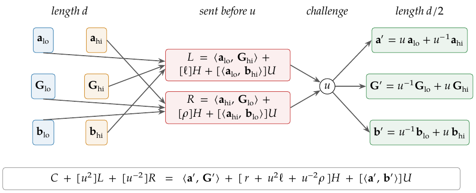
The four cross inner products $\langle\mathbf{a}_{\mathrm{lo}},\,\mathbf{G}_{\mathrm{hi}}\rangle$ , $\langle\mathbf{a}_{\mathrm{hi}},\,\mathbf{G}_{\mathrm{lo}}\rangle$ , $\langle\mathbf{a}_{\mathrm{lo}},\,\mathbf{b}_{\mathrm{hi}}\rangle$ and $\langle\mathbf{a}_{\mathrm{hi}},\,\mathbf{b}_{\mathrm{lo}}\rangle$ involve only the halves, not $u$ . The prover can therefore commit to them before the challenge is drawn. She samples two fresh blinders $\ell,\rho\in\mathbb{F}$ and sends the two group elements

L:=\langle\mathbf{a}_{\mathrm{lo}},\,\mathbf{G}_{\mathrm{hi}}\rangle+[\ell]H+[% \langle\mathbf{a}_{\mathrm{lo}},\,\mathbf{b}_{\mathrm{hi}}\rangle]\,U,\qquad R% :=\langle\mathbf{a}_{\mathrm{hi}},\,\mathbf{G}_{\mathrm{lo}}\rangle+[\rho]H+[% \langle\mathbf{a}_{\mathrm{hi}},\,\mathbf{b}_{\mathrm{lo}}\rangle]\,U,

(13)

each of the same three-part shape as $C$ : a vector part on the generators, a blinder on $H$ , and the matching scalar inner product on $U$ . Only then does the verifier draw $u$ .

The fold identity.

Now add the cross terms to $C$ with the weights the expansion produced and regroup by generator set:

	$\displaystyle C+[u^{2}]L+[u^{-2}]R$	$\displaystyle=\langle\mathbf{a},\,\mathbf{G}\rangle+[r]H+[\langle\mathbf{a},\,% \mathbf{b}\rangle]\,U$
		$\displaystyle\quad+u^{2}\Bigl{(}\langle\mathbf{a}_{\mathrm{lo}},\,\mathbf{G}_{% \mathrm{hi}}\rangle+[\ell]H+[\langle\mathbf{a}_{\mathrm{lo}},\,\mathbf{b}_{% \mathrm{hi}}\rangle]\,U\Bigr{)}$
		$\displaystyle\quad+u^{-2}\Bigl{(}\langle\mathbf{a}_{\mathrm{hi}},\,\mathbf{G}_% {\mathrm{lo}}\rangle+[\rho]H+[\langle\mathbf{a}_{\mathrm{hi}},\,\mathbf{b}_{% \mathrm{lo}}\rangle]\,U\Bigr{)}$
		$\displaystyle=\Bigl{(}\langle\mathbf{a},\,\mathbf{G}\rangle+u^{2}\langle% \mathbf{a}_{\mathrm{lo}},\,\mathbf{G}_{\mathrm{hi}}\rangle+u^{-2}\langle% \mathbf{a}_{\mathrm{hi}},\,\mathbf{G}_{\mathrm{lo}}\rangle\Bigr{)}$
		$\displaystyle\quad+[\,r+u^{2}\ell+u^{-2}\rho\,]H+\Bigl{[}\langle\mathbf{a},\,% \mathbf{b}\rangle+u^{2}\langle\mathbf{a}_{\mathrm{lo}},\,\mathbf{b}_{\mathrm{% hi}}\rangle+u^{-2}\langle\mathbf{a}_{\mathrm{hi}},\,\mathbf{b}_{\mathrm{lo}}% \rangle\Bigr{]}\,U$
		$\displaystyle=\langle\mathbf{a}^{\prime},\,\mathbf{G}^{\prime}\rangle+[r^{% \prime}]H+[\langle\mathbf{a}^{\prime},\,\mathbf{b}^{\prime}\rangle]\,U,$

where $r^{\prime}:=r+u^{2}\ell+u^{-2}\rho$ and the last line substitutes the two expansions. Written as one equation, the fold identity is

C^{\prime}:=C+[u^{2}]L+[u^{-2}]R=\langle\mathbf{a}^{\prime},\,\mathbf{G}^{% \prime}\rangle+[r^{\prime}]H+[\langle\mathbf{a}^{\prime},\,\mathbf{b}^{\prime}% \rangle]\,U.

(14)

What has been achieved.

Compare the two sides of (14) with (11). The element $C^{\prime}$ has the same shape as $C$ , over vectors of half the length: its $\mathbf{G}^{\prime}$ -part is the folded coefficient vector, its $H$ -part a blinder, and its $U$ -coefficient the inner product of the folded vectors. The verifier can compute $C^{\prime}$ , $\mathbf{G}^{\prime}$ and $\mathbf{b}^{\prime}$ entirely on his own from $C$ , $L$ , $R$ , $u$ and the public data. The prover computes $\mathbf{a}^{\prime}$ and $r^{\prime}$ . The claim about $(\mathbf{a},\mathbf{b},\mathbf{G})$ of length $d$ has been replaced by a claim about $(\mathbf{a}^{\prime},\mathbf{b}^{\prime},\mathbf{G}^{\prime})$ of length $d/2$ , and the exchange cost exactly two group elements and one field element of challenge. Figure 7 shows the fold and identity (14). Only completeness is claimed here; that a prover who cannot open $C$ cannot open $C^{\prime}$ either is proved in §3.5.

The evaluation vector folds into a power vector.

When $\mathbf{b}=\mathbf{b}(x)$ , the high half is the low half scaled: $\mathbf{b}_{\mathrm{hi}}=x^{d/2}\,\mathbf{b}_{\mathrm{lo}}$ , since $b_{i+d/2}=x^{i+d/2}=x^{d/2}x^{i}$ . Hence

\mathbf{b}^{\prime}=u^{-1}\mathbf{b}_{\mathrm{lo}}+u\,x^{d/2}\mathbf{b}_{% \mathrm{lo}}=\bigl{(}u^{-1}+u\,x^{d/2}\bigr{)}\,(1,x,\dots,x^{d/2-1}):

the folded evaluation vector is again a vector of powers of $x$ , scaled by the scalar $u^{-1}+ux^{d/2}$ . The verifier never needs to store $\mathbf{b}^{\prime}$ ; he needs one scalar per round. This is the seed of the closed form $g$ of §3.4.

The fold at $d=4$ , symbolically.

For the running example’s length, the halves are $\mathbf{a}_{\mathrm{lo}}=(a_{0},a_{1})$ , $\mathbf{a}_{\mathrm{hi}}=(a_{2},a_{3})$ , $\mathbf{G}_{\mathrm{lo}}=(G_{0},G_{1})$ , $\mathbf{G}_{\mathrm{hi}}=(G_{2},G_{3})$ , $\mathbf{b}_{\mathrm{lo}}=(1,x)$ and $\mathbf{b}_{\mathrm{hi}}=(x^{2},x^{3})$ , so the cross terms of (13) read

	$\displaystyle L$	$\displaystyle=[a_{0}]G_{2}+[a_{1}]G_{3}+[\ell]H+[a_{0}x^{2}+a_{1}x^{3}]\,U,$
	$\displaystyle R$	$\displaystyle=[a_{2}]G_{0}+[a_{3}]G_{1}+[\rho]H+[a_{2}+a_{3}x]\,U,$

and the folded vectors are $\mathbf{a}^{\prime}=(ua_{0}+u^{-1}a_{2},\;ua_{1}+u^{-1}a_{3})$ , $\mathbf{G}^{\prime}=([u^{-1}]G_{0}+[u]G_{2},\;[u^{-1}]G_{1}+[u]G_{3})$ and $\mathbf{b}^{\prime}=(u^{-1}+ux^{2})\,(1,x)$ . Section 3.7 fills these in with numbers.

Refer to caption — Figure 7: One fold. The three vectors of length $d$ (left; low halves in blue, high halves in amber) determine the two cross terms $L$ and $R$ (red): $L$ from $\mathbf{a}_{\mathrm{lo}}$ , $\mathbf{G}_{\mathrm{hi}}$ and $\mathbf{b}_{\mathrm{hi}}$ , $R$ from the complementary halves, both sent before the challenge $u$ is drawn. The challenge then folds all three vectors to length $d/2$ (green). The identity beneath is equation (14): the folded commitment has the same three-part shape as the original, over the folded vectors, with the cross terms absorbed at weights $u^{2}$ and $u^{-2}$ .

3.3 The recursion: $k$ rounds to a single scalar

The folded claim of §3.2 has the shape of the original claim, so it can be folded again. After $k=\log_{2}d$ folds the vectors have length one, and a length-one claim is checked by sending the scalar and its blinder. That is the whole protocol; this subsection writes it out as a construction, numbers the rounds, and lays the two parties’ work side by side.

Construction 3.2 (IPA-based polynomial commitment).

Let $\mathbb{G}$ be a cyclic group of prime order $p$ in which the discrete logarithm problem is hard (Crypto Guide, §“Standing assumptions”), and let $\mathbb{F}=\mathbb{F}_{p}$ . Choose $d=2^{k}$ and sample the generators $\mathbf{G}=(G_{0},\dots,G_{d-1})$ and $H$ independently and uniformly from $\mathbb{G}\setminus\{\mathcal{O}\}$ , as in the Crypto Guide’s Construction “Pedersen vector commitment” (§“Pedersen vector commitments”). Deployed generators are instead hash-to-curve outputs on public labels, uniform when hash-to-curve is modelled as a random oracle into $\mathbb{G}$ (Crypto Guide, §“Hashing to a curve point”, Remark “Why NUMS generators are binding-safe”).

Commitment. For $p(X)=\sum_{i=0}^{d-1}a_{i}X^{i}\in\mathbb{F}[X]$ and a blinder $r\in\mathbb{F}$ ,

\mathsf{Commit}(p;\,r):=\langle\mathbf{a},\,\mathbf{G}\rangle+[r]H\in\mathbb{G}.

Opening. To prove $((P,x,v);(\mathbf{a},r))\in\mathcal{R}_{\mathrm{IPA}}$ , the two parties proceed as follows.

1.

Setup. The verifier samples $U$ uniformly from $\mathbb{G}\setminus\{\mathcal{O}\}$ and sends it. Both parties set $C^{(k)}:=P+[v]U$ , $\mathbf{G}^{(k)}:=\mathbf{G}$ and $\mathbf{b}^{(k)}:=\mathbf{b}(x)$ ; the prover sets $\mathbf{a}^{(k)}:=\mathbf{a}$ and $r^{(k)}:=r$ .
2.
Rounds. For $j=k,k-1,\dots,1$ , the vectors $\mathbf{a}^{(j)},\mathbf{G}^{(j)},\mathbf{b}^{(j)}$ have length $2^{j}$ and are split into halves as in §3.2.
1. (a)
  
  The prover samples independent uniform $\ell_{j},\rho_{j}\in\mathbb{F}$ and sends
  
  $\displaystyle L_{j}$ $\displaystyle:=\langle\mathbf{a}^{(j)}_{\mathrm{lo}},\,\mathbf{G}^{(j)}_{% \mathrm{hi}}\rangle+[\ell_{j}]H+[\langle\mathbf{a}^{(j)}_{\mathrm{lo}},\,% \mathbf{b}^{(j)}_{\mathrm{hi}}\rangle]\,U,$
  
  $\displaystyle R_{j}$ $\displaystyle:=\langle\mathbf{a}^{(j)}_{\mathrm{hi}},\,\mathbf{G}^{(j)}_{% \mathrm{lo}}\rangle+[\rho_{j}]H+[\langle\mathbf{a}^{(j)}_{\mathrm{hi}},\,% \mathbf{b}^{(j)}_{\mathrm{lo}}\rangle]\,U.$
2. (b)
  
  The verifier sends a uniform $u_{j}\in\mathbb{F}^{\times}$ .
3. (c)
  
  Both parties fold by (12):
  
  $\displaystyle\mathbf{G}^{(j-1)}:=u_{j}^{-1}\mathbf{G}^{(j)}_{\mathrm{lo}}+u_{j% }\,\mathbf{G}^{(j)}_{\mathrm{hi}},\qquad\mathbf{b}^{(j-1)}:=u_{j}^{-1}\mathbf{% b}^{(j)}_{\mathrm{lo}}+u_{j}\,\mathbf{b}^{(j)}_{\mathrm{hi}},$
  
  $\displaystyle C^{(j-1)}:=C^{(j)}+[u_{j}^{2}]L_{j}+[u_{j}^{-2}]R_{j};$
  
  the prover also folds $\mathbf{a}^{(j-1)}:=u_{j}\,\mathbf{a}^{(j)}_{\mathrm{lo}}+u_{j}^{-1}\mathbf{a}% ^{(j)}_{\mathrm{hi}}$ and $r^{(j-1)}:=r^{(j)}+u_{j}^{2}\ell_{j}+u_{j}^{-2}\rho_{j}$ .
3.

Final message. After round $1$ every vector has length one. Write $a:=\mathbf{a}^{(0)}$ , $G^{(0)}:=\mathbf{G}^{(0)}$ and $b^{(0)}:=\mathbf{b}^{(0)}$ for the single entries. The prover sends the scalar $a$ and the aggregated blinder

$r^{*}:=r^{(0)}=r+\sum_{j=1}^{k}\bigl{(}u_{j}^{2}\,\ell_{j}+u_{j}^{-2}\rho_{j}% \bigr{)}.$
4.

Check. The verifier accepts if and only if

$P+[v]U+\sum_{j=1}^{k}\bigl{(}[u_{j}^{2}]L_{j}+[u_{j}^{-2}]R_{j}\bigr{)}\;% \overset{?}{=}\;[a]\,G^{(0)}+[r^{*}]H+[a\cdot b^{(0)}]\,U,$ (15)

where the left-hand side is $C^{(0)}$ and $G^{(0)}$ , $b^{(0)}$ are computed as §3.4 describes.

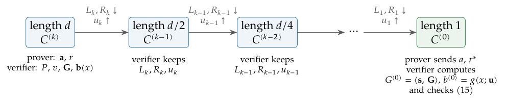
The round index descends so that round $j$ begins with vectors of length $2^{j}$ ; round $k$ is the first round and round $1$ the last. The scheme instantiates the polynomial-commitment interface of the Crypto Guide (§“Polynomial commitment schemes”, the inner-product alternative), and the opening protocol is the inner-product argument of Bootle, Cerulli, Chaidos, Groth and Petit as refined in Bulletproofs by Bünz, Bootle, Boneh, Poelstra, Wuille and Maxwell, in the symmetric normalisation those papers use.

Completeness.

The honest prover always passes. By induction on the rounds,

C^{(j)}=\langle\mathbf{a}^{(j)},\,\mathbf{G}^{(j)}\rangle+[r^{(j)}]H+[\langle% \mathbf{a}^{(j)},\,\mathbf{b}^{(j)}\rangle]\,U\qquad\text{for }j=k,k-1,\dots,0:

(16)

at $j=k$ this is (11) with the honest $P$ , and the step from $j$ to $j-1$ is the fold identity (14) applied to the round’s vectors, challenge and blinders. At $j=0$ the vectors have one entry each, the inner products are products of scalars, and (16) reads $C^{(0)}=[a]G^{(0)}+[r^{*}]H+[a\,b^{(0)}]U$ , which is (15). The only way an honest run can fail is a challenge $u_{j}=0$ , which the verifier excludes.

Proof size.

The prover sends two group elements per round and two field elements at the end: $2k$ group elements plus $O(1)$ , against the $d+1=2^{k}+1$ field elements of the trivial protocol. The verifier keeps only the challenges $u_{1},\dots,u_{k}$ and the received points; he need not fold $\mathbf{G}$ round by round, as the next subsection shows. Figure 8 draws the $k$ rounds, and Tables 2 and 3 list, one row per message, what each party holds, computes and sends, so that a reader can play either role; §3.7 refills the same rows with numbers.

step	receives / holds	computes and sends
setup	holds $\mathbf{a}$ , $r$ , $x$ , $v$ ; receives $U$	sets $\mathbf{a}^{(k)}:=\mathbf{a}$ , $\mathbf{G}^{(k)}:=\mathbf{G}$ , $\mathbf{b}^{(k)}:=\mathbf{b}(x)$ , $r^{(k)}:=r$
round $j$	vectors of length $2^{j}$ , split into halves	samples $\ell_{j},\rho_{j}$ ; sends $L_{j}$ , $R_{j}$ as in Construction 3.2
	receives $u_{j}$	folds $\mathbf{a}^{(j-1)}=u_{j}\mathbf{a}^{(j)}_{\mathrm{lo}}+u_{j}^{-1}\mathbf{a}^{(% j)}_{\mathrm{hi}}$ , $\mathbf{G}^{(j-1)}$ , $\mathbf{b}^{(j-1)}$ ; $r^{(j-1)}=r^{(j)}+u_{j}^{2}\ell_{j}+u_{j}^{-2}\rho_{j}$
final	one entry each: $a=\mathbf{a}^{(0)}$ , $r^{*}=r^{(0)}$	sends $a$ , $r^{*}$

Table 2: The prover’s side of Construction 3.2, one row per message. The round row repeats for

j=k,\dots,1

step	receives / holds	computes and sends
setup	holds $P$ , $x$ , $v$ , $\mathbf{G}$ , $H$	samples $U$ and sends it; sets $C^{(k)}:=P+[v]U$
round $j$	receives $L_{j}$ , $R_{j}$	samples $u_{j}\in\mathbb{F}^{\times}$ and sends it; keeps $(L_{j},R_{j},u_{j})$ ; optionally $C^{(j-1)}:=C^{(j)}+[u_{j}^{2}]L_{j}+[u_{j}^{-2}]R_{j}$
final	receives $a$ , $r^{*}$	computes $\mathbf{s}$ and $G^{(0)}=\langle\mathbf{s},\,\mathbf{G}\rangle$ (one length- $d$ multi-scalar multiplication), $b^{(0)}=g(x;u_{1},\dots,u_{k})$ ( $O(k)$ field operations), and checks (15)

Table 3: The verifier’s side of Construction 3.2, one row per message, with the closing computations of §3.4. The round row repeats for

j=k,\dots,1

; folding

C

round by round is optional because (15) sums the cross terms directly.

3.4 The verifier’s work: structured scalars and the final generator

The check (15) needs two quantities the verifier has not yet been told how to obtain cheaply: the final generator $G^{(0)}$ and the final evaluation scalar $b^{(0)}$ . Folding $\mathbf{G}$ round by round costs $d+d/2+\dots+2=2d-2$ scalar multiplications (two per entry of each folded vector), and folding $\mathbf{b}$ likewise many field operations. Both have closed forms in the challenges.

Theorem 3.3 (Structured scalars and the polynomial $g$ ).

For $0\leq i<d$ write the binary expansion $i=\sum_{\ell=0}^{k-1}\beta_{\ell}\,2^{\ell}$ with digits $\beta_{\ell}\in\{0,1\}$ , and define the structured scalars

s_{i}:=\prod_{\ell=1}^{k}u_{\ell}^{\,(-1)^{1-\beta_{\ell-1}}}\qquad\text{(the % factor is $u_{\ell}$ when }\beta_{\ell-1}=1\text{ and }u_{\ell}^{-1}\text{ % when }\beta_{\ell-1}=0\text{)}.

(17)

Then, after the $k$ folds of Construction 3.2,

G^{(0)}=\langle\mathbf{s},\,\mathbf{G}\rangle=\sum_{i=0}^{d-1}[s_{i}]\,G_{i},% \qquad b^{(0)}=\langle\mathbf{s},\,\mathbf{b}(x)\rangle=g(x;\,u_{1},\dots,u_{k% }),

(18)

where

g(X;\,u_{1},\dots,u_{k}):=\prod_{\ell=1}^{k}\bigl{(}u_{\ell}^{-1}+u_{\ell}\,X^% {2^{\ell-1}}\bigr{)},

(19)

a polynomial of degree $d-1$ in $X$ .

Proof.

Follow one original generator $G_{m}$ through the folds. Claim: after the rounds $k,k-1,\dots,j+1$ have been performed, $G_{m}$ contributes to exactly one entry of $\mathbf{G}^{(j)}$ , the entry at position $m\bmod 2^{j}$ , with coefficient $\prod_{\ell=j+1}^{k}u_{\ell}^{(-1)^{1-\beta_{\ell-1}}}$ , where $\beta_{\ell-1}$ is the digit of $m$ at position $\ell-1$ . At $j=k$ nothing has happened and the claim says $G_{m}$ sits at position $m$ with coefficient $1$ . For the step from $j$ to $j-1$ : round $j$ folds the length- $2^{j}$ vector by $G^{(j-1)}_{i}=[u_{j}^{-1}]G^{(j)}_{i}+[u_{j}]G^{(j)}_{i+2^{j-1}}$ for $0\leq i<2^{j-1}$ . The position $m\bmod 2^{j}$ lies in the low half $[0,2^{j-1})$ exactly when the digit $\beta_{j-1}$ of $m$ is $0$ , in which case it moves to position $m\bmod 2^{j-1}$ with the extra factor $u_{j}^{-1}$ ; and it lies in the high half exactly when $\beta_{j-1}=1$ , in which case it is the entry $i+2^{j-1}$ with $i=m\bmod 2^{j-1}$ and moves to position $i$ with the extra factor $u_{j}$ . Either way the new coefficient is the old one times $u_{j}^{(-1)^{1-\beta_{j-1}}}$ , which is the claim for $j-1$ . At $j=0$ every $G_{m}$ sits in the single entry $G^{(0)}$ with coefficient $s_{m}$ , which is the first half of (18). The vector $\mathbf{b}$ is folded with the same weights, so the same argument gives $b^{(0)}=\sum_{m}s_{m}\,b_{m}=\langle\mathbf{s},\,\mathbf{b}(x)\rangle$ .

For the closed form, expand the product (19): choosing from the $\ell$ -th factor either $u_{\ell}^{-1}$ (when $\beta_{\ell-1}=0$ ) or $u_{\ell}X^{2^{\ell-1}}$ (when $\beta_{\ell-1}=1$ ) produces, for each $m$ , the monomial $s_{m}X^{\sum_{\ell=1}^{k}\beta_{\ell-1}2^{\ell-1}}=s_{m}X^{m}$ , and every $m\in[0,d)$ arises from exactly one choice. Hence $g(X)=\sum_{m}s_{m}X^{m}$ , whose value at $x$ is $\langle\mathbf{s},\,\mathbf{b}(x)\rangle$ , and whose degree is $d-1$ since the top monomial has coefficient $s_{d-1}=\prod_{\ell}u_{\ell}\neq 0$ . □

At $d=4$ the scalars are $s_{0}=u_{1}^{-1}u_{2}^{-1}$ , $s_{1}=u_{1}u_{2}^{-1}$ , $s_{2}=u_{1}^{-1}u_{2}$ and $s_{3}=u_{1}u_{2}$ , and $g(x;u_{1},u_{2})=(u_{1}^{-1}+u_{1}x)(u_{2}^{-1}+u_{2}x^{2})$ : the digit of weight $1$ selects the exponent of $u_{1}$ , the round that folded pairs of neighbours, and the digit of weight $2$ selects the exponent of $u_{2}$ , the round that folded the two halves of the whole vector.

The final equation, and why it checks.

The verifier’s closing work is now explicit. He evaluates $b^{(0)}=g(x;\mathbf{u})$ from the challenges; he computes $G^{(0)}=\langle\mathbf{s},\,\mathbf{G}\rangle$ , one multi-scalar multiplication of length $d$ ; he adds up the left-hand side of (15) from $P$ , $U$ , the $2k$ received points and the challenges, $2k+1$ scalar multiplications; and he compares it with the right-hand side, three more scalar multiplications. For the honest prover the two sides agree by the invariant (16). That a dishonest prover cannot make them agree except by knowing an opening is §3.5.

The cost of the final check.

Evaluating $g$ at $x$ costs $3k-2$ field multiplications: $k$ products $u_{\ell}\,x^{2^{\ell-1}}$ , $k-1$ squarings to produce the powers $x,x^{2},x^{4},\dots$ , and $k-1$ multiplications of the factors together; at $k=2$ that is four multiplications, and at Orchard’s $k=11$ it is $31$ . But $G^{(0)}$ is a linear combination of all $d$ generators, and computing it is a multi-scalar multiplication of length $d$ , at Orchard’s $d=2^{11}$ some $2048$ scalar multiplications: the one part of the verifier’s work that is linear in the size of the committed vector, and the check “linear in $n$ ” that §2.6 deferred to this subsection. Everything else the verifier does is logarithmic. The asymmetry has a name in the closed form: $G^{(0)}=\langle\mathbf{s},\,\mathbf{G}\rangle$ is nothing but $\mathsf{Commit}(g;\,0)$ , the unblinded commitment to the polynomial $g$ whose value the verifier just computed in $O(k)$ operations. Checking a value of $g$ is cheap; checking its commitment is not. This asymmetry is the seed of the accumulation scheme of §7, and of the deferral described at the end of this section.

3.5 Why it is binding: extraction from three transcripts

This subsection shows that any prover that makes the verifier of Construction 3.2 accept knows an opening $(\mathbf{a},r)$ of $P$ with $\langle\mathbf{a},\,\mathbf{b}(x)\rangle=v$ , in the operational sense of the Crypto Guide (§“Knowledge soundness and extractors”): an extractor that runs the prover as a subroutine, rewinds it to an earlier state and feeds it fresh challenges computes the pair from its answers. The mechanism is the one that makes Schnorr’s identification protocol a proof of knowledge (Crypto Guide, §“The Schnorr identification protocol”): a single transcript reveals nothing, but two accepting transcripts with the same first message and distinct challenges are two linear equations, and subtracting them cancels the unknown commitment and leaves the witness. Here each round has three unknown group elements instead of one, so three transcripts are needed per round, and the $k$ rounds stack the three-way branching into a tree, the tree special soundness of the Crypto Guide (§“Sigma-protocols”). The single-round step is pure linear algebra and is proved in full; the tree is an induction on it; the discrete-logarithm assumption enters once, at the root.

Representations.

Fix a level $j$ with generator vector $\mathbf{G}^{(j)}$ of length $2^{j}$ . A representation of an element $Q\in\mathbb{G}$ over $(\mathbf{G}^{(j)},H,U)$ is a triple $(\mathbf{x};y;w)\in\mathbb{F}^{2^{j}}\times\mathbb{F}\times\mathbb{F}$ with

Q=\langle\mathbf{x},\,\mathbf{G}^{(j)}\rangle+[y]H+[w]U.

Call the representation well formed at level $j$ if its $U$ -coordinate is the inner product of its $\mathbf{G}$ -coordinates with the round’s evaluation vector, $w=\langle\mathbf{x},\,\mathbf{b}^{(j)}\rangle$ . The invariant (16) says exactly that the honest prover holds a well-formed representation $(\mathbf{a}^{(j)};r^{(j)};\langle\mathbf{a}^{(j)},\,\mathbf{b}^{(j)}\rangle)$ of $C^{(j)}$ at every level. A representation over folded generators lifts to one over the generators of the level above: if $Q=\langle\mathbf{a}^{\prime},\,\mathbf{G}^{\prime}\rangle+[y]H+[w]U$ with $\mathbf{G}^{\prime}=u^{-1}\mathbf{G}_{\mathrm{lo}}+u\,\mathbf{G}_{\mathrm{hi}}$ , then by bilinearity

Q=\langle(u^{-1}\mathbf{a}^{\prime},\;u\,\mathbf{a}^{\prime}),\,\mathbf{G}% \rangle+[y]H+[w]U,

(20)

and the lift preserves well-formedness, since $\langle(u^{-1}\mathbf{a}^{\prime},u\mathbf{a}^{\prime}),\,\mathbf{b}\rangle=% \langle\mathbf{a}^{\prime},\,u^{-1}\mathbf{b}_{\mathrm{lo}}+u\,\mathbf{b}_{% \mathrm{hi}}\rangle=\langle\mathbf{a}^{\prime},\,\mathbf{b}^{\prime}\rangle$ . Under the discrete-logarithm assumption a prover can know at most one representation of any $Q$ : two of them differ by a nontrivial relation among $\mathbf{G}$ , $H$ and $U$ , which is the binding argument of the Crypto Guide (§“Pedersen vector commitments”). Nothing below uses this until the root is reached.

Lemma 3.4 (Single-round recovery).

Fix one round of Construction 3.2 at level $j$ : the verifier’s element $C:=C^{(j)}$ , the generators $\mathbf{G}:=\mathbf{G}^{(j)}$ and evaluation vector $\mathbf{b}:=\mathbf{b}^{(j)}$ , and the prover’s cross terms $L$ , $R$ . Let $u,u^{\prime},u^{\prime\prime}$ be three challenges for this round, and suppose that for each $\nu\in\{u,u^{\prime},u^{\prime\prime}\}$ a representation $(\mathbf{x}_{\nu};y_{\nu};w_{\nu})$ of the folded element $C+[\nu^{2}]L+[\nu^{-2}]R$ over $(\mathbf{G},H,U)$ is known. If the squares $u^{2},u^{\prime 2},u^{\prime\prime 2}$ are pairwise distinct, then representations $(\mathbf{x}_{L};y_{L};w_{L})$ , $(\mathbf{x}_{C};y_{C};w_{C})$ and $(\mathbf{x}_{R};y_{R};w_{R})$ of $L$ , $C$ and $R$ over $(\mathbf{G},H,U)$ are obtained by solving one $3\times 3$ linear system with rows $(\nu^{2},1,\nu^{-2})$ , and they satisfy, for each $\nu$ ,

\mathbf{x}_{\nu}=\nu^{2}\mathbf{x}_{L}+\mathbf{x}_{C}+\nu^{-2}\mathbf{x}_{R},% \qquad y_{\nu}=\nu^{2}y_{L}+y_{C}+\nu^{-2}y_{R},\qquad w_{\nu}=\nu^{2}w_{L}+w_% {C}+\nu^{-2}w_{R}.

(21)

If the three given representations are well formed at level $j$ , so is the recovered representation of $C$ .

Proof.

Write the three known representations as vectors $\mathbf{Y}_{\nu}:=(\mathbf{x}_{\nu},y_{\nu},w_{\nu})\in\mathbb{F}^{2^{j}+2}$ and the three unknown ones as $\mathbf{X}_{L},\mathbf{X}_{C},\mathbf{X}_{R}$ . The three group equations

[\nu^{2}]L+C+[\nu^{-2}]R=\langle\mathbf{x}_{\nu},\,\mathbf{G}\rangle+[y_{\nu}]% H+[w_{\nu}]U,\qquad\nu\in\{u,u^{\prime},u^{\prime\prime}\},

suggest the linear system

M\begin{pmatrix}\mathbf{X}_{L}\\ \mathbf{X}_{C}\\ \mathbf{X}_{R}\end{pmatrix}=\begin{pmatrix}\mathbf{Y}_{u}\\ \mathbf{Y}_{u^{\prime}}\\ \mathbf{Y}_{u^{\prime\prime}}\end{pmatrix},\qquad M:=\begin{pmatrix}u^{2}&1&u^% {-2}\\ u^{\prime 2}&1&u^{\prime-2}\\ u^{\prime\prime 2}&1&u^{\prime\prime-2}\end{pmatrix},

to be solved coordinate by coordinate. Multiplying the row of $\nu$ by the nonzero scalar $\nu^{2}$ turns it into $(\nu^{4},\nu^{2},1)$ , which does not change the kernel. If $M(c_{0},c_{1},c_{2})^{\top}=0$ , the polynomial $c_{0}W^{2}+c_{1}W+c_{2}$ of degree at most $2$ vanishes at $W=u^{2},u^{\prime 2},u^{\prime\prime 2}$ ; when these squares are pairwise distinct it is zero (Math Guide, §“Roots and the factor theorem”, Theorem “At most $d$ roots”), so $M$ is invertible. When two squares coincide, two rows of $M$ coincide and $M$ is singular. Define $(\mathbf{X}_{L},\mathbf{X}_{C},\mathbf{X}_{R})$ as the unique solution. Because it solves the system exactly, $\mathbf{Y}_{\nu}=\nu^{2}\mathbf{X}_{L}+\mathbf{X}_{C}+\nu^{-2}\mathbf{X}_{R}$ for each $\nu$ , which is (21) read coordinate by coordinate. That the solutions are representations of $L$ , $C$ and $R$ follows by taking the same linear combinations of the group equations: let $(\alpha,\alpha^{\prime},\alpha^{\prime\prime})$ be the middle row of $M^{-1}$ , so that $\alpha(u^{2},1,u^{-2})+\alpha^{\prime}(u^{\prime 2},1,u^{\prime-2})+\alpha^{% \prime\prime}(u^{\prime\prime 2},1,u^{\prime\prime-2})=(0,1,0)$ and $\mathbf{X}_{C}=\alpha\mathbf{Y}_{u}+\alpha^{\prime}\mathbf{Y}_{u^{\prime}}+% \alpha^{\prime\prime}\mathbf{Y}_{u^{\prime\prime}}$ . Adding $\alpha$ times the first group equation, $\alpha^{\prime}$ times the second and $\alpha^{\prime\prime}$ times the third gives, on the left, $[0]L+[1]C+[0]R=C$ , and on the right, by bilinearity, $\langle\mathbf{x}_{C},\,\mathbf{G}\rangle+[y_{C}]H+[w_{C}]U$ . The first and third rows of $M^{-1}$ do the same for $L$ and $R$ . For well-formedness, set $\delta_{\nu}:=w_{\nu}-\langle\mathbf{x}_{\nu},\,\mathbf{b}\rangle$ and $\delta_{L}:=w_{L}-\langle\mathbf{x}_{L},\,\mathbf{b}\rangle$ , $\delta_{C}:=w_{C}-\langle\mathbf{x}_{C},\,\mathbf{b}\rangle$ , $\delta_{R}:=w_{R}-\langle\mathbf{x}_{R},\,\mathbf{b}\rangle$ . Subtracting the inner product of the first identity of (21) with $\mathbf{b}$ from the third gives $\delta_{\nu}=\nu^{2}\delta_{L}+\delta_{C}+\nu^{-2}\delta_{R}$ for each $\nu$ , that is, $M(\delta_{L},\delta_{C},\delta_{R})^{\top}=(\delta_{u},\delta_{u^{\prime}},% \delta_{u^{\prime\prime}})^{\top}$ . If the given representations are well formed the right-hand side is zero, and $M$ invertible forces $\delta_{L}=\delta_{C}=\delta_{R}=0$ ; in particular $w_{C}=\langle\mathbf{x}_{C},\,\mathbf{b}\rangle$ . □

Theorem 3.5 (Knowledge soundness of the opening protocol).

Let $\mathbb{G}$ be a group of prime order in which the discrete logarithm problem is hard, and let $\mathbf{G}$ and $H$ be uniform in $\mathbb{G}\setminus\{\mathcal{O}\}$ as in Construction 3.2 (for hashed generators: hash-to-curve modelled as a random oracle into $\mathbb{G}$ ). The opening protocol of Construction 3.2 is knowledge sound for $\mathcal{R}_{\mathrm{IPA}}$ : there is an extractor which, given rewindable access to any prover that makes the verifier accept with non-negligible probability, runs in expected polynomial time and outputs either a witness $(\mathbf{a},r)$ with $P=\langle\mathbf{a},\,\mathbf{G}\rangle+[r]H$ and $\langle\mathbf{a},\,\mathbf{b}(x)\rangle=v$ , or a nontrivial discrete-logarithm relation among $\mathbf{G}$ , $H$ and the verifier’s generators $U$ , $U^{\prime}$ . Its knowledge error is $O(\log d/|\mathbb{F}|)$ .

Proof.

The proof is given at the level of this volume: the single-round step is Lemma 3.4, the tree is an induction on it, and the rewinding that supplies the sibling transcripts is the Crypto Guide’s (§“The Schnorr identification protocol”, the remark on extraction by rewinding, and §“Sigma-protocols”, the tree-extraction theorem cited there, which also gives the expected running time). The trees it assembles have children with pairwise distinct challenges (the Crypto Guide’s Definition “Tree special soundness”), while Lemma 3.4 needs pairwise distinct squares. A square has at most two square roots, so any five pairwise distinct challenges contain three with pairwise distinct squares: the rewinding assembles five children per node, and the extractor uses three of them. From a tree the extractor computes a witness or, at the root, a discrete-logarithm relation; that definition asks for a witness alone, and the difference is where the assumption enters.

Leaves. Rewind the prover to the moment after it sent $(L_{1},R_{1})$ and obtain three accepting final messages $(a,r^{*})$ for three challenges $u_{1}$ with pairwise distinct squares. An accepting final message is, by (15), a representation of $C^{(0)}$ over $(G^{(0)},H,U)$ , namely $(a;r^{*};a\,b^{(0)})$ , and it is well formed at level $0$ : its $U$ -coordinate is the inner product of $a$ with the length-one vector $b^{(0)}$ . Lift it to level $1$ by (20): $\mathbf{x}=(u_{1}^{-1}a,u_{1}a)$ .

One node. The three lifted leaves are well-formed representations of the three folded elements $C^{(1)}+[u_{1}^{2}]L_{1}+[u_{1}^{-2}]R_{1}$ over $(\mathbf{G}^{(1)},H,U)$ . Lemma 3.4 at the round- $1$ node returns a well-formed representation of $C^{(1)}$ (and representations of $L_{1}$ and $R_{1}$ , which are not needed further).

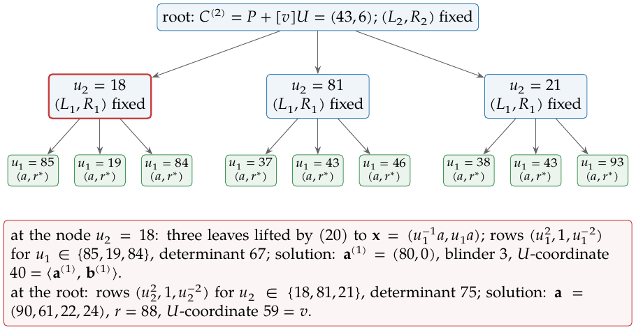
Induction. Rewind to the moment after $(L_{2},R_{2})$ , obtain three challenges $u_{2}$ with pairwise distinct squares, and under each of them repeat the two steps above. That yields, after lifting to level $2$ , three well-formed representations of the elements $C^{(2)}+[u_{2}^{2}]L_{2}+[u_{2}^{-2}]R_{2}$ , and the lemma at the round- $2$ node returns a well-formed representation of $C^{(2)}$ . Continuing upward, after $k$ levels the extractor holds a well-formed representation $(\mathbf{x};y;w)$ of $C^{(k)}=P+[v]U$ over $(\mathbf{G},H,U)$ , with $w=\langle\mathbf{x},\,\mathbf{b}(x)\rangle$ . The tree of transcripts consumed has three children at every node and depth $k$ , hence $3^{k}=d^{\log_{2}3}$ leaves (Figure 9).

The root, where the assumption enters. The root representation says $P=\langle\mathbf{x},\,\mathbf{G}\rangle+[y]H+[w-v]U$ . If $w=v$ then $(\mathbf{x},y)$ is a witness: $P=\langle\mathbf{x},\,\mathbf{G}\rangle+[y]H$ and $\langle\mathbf{x},\,\mathbf{b}(x)\rangle=w=v$ . If $w\neq v$ , the extractor rewinds once more, to the setup step at which the verifier sampled $U$ , and repeats the whole extraction under an independent sample $U^{\prime}$ , obtaining $P=\langle\mathbf{x}^{\prime},\,\mathbf{G}\rangle+[y^{\prime}]H+[w^{\prime}-v]U% ^{\prime}$ . If $w^{\prime}=v$ the witness is $(\mathbf{x}^{\prime},y^{\prime})$ . Otherwise subtracting the two expressions for $P$ gives

[w-v]\,U-[w^{\prime}-v]\,U^{\prime}+\langle\mathbf{x}-\mathbf{x}^{\prime},\,% \mathbf{G}\rangle+[y-y^{\prime}]H=\mathcal{O}

with the nonzero coefficient $w-v$ on $U$ : a nontrivial relation among the independent uniform generators $\mathbf{G}$ , $H$ , $U$ , $U^{\prime}$ , which the every-generator embedding of the Crypto Guide (§“Pedersen vector commitments”, the proof of binding) turns into a discrete logarithm, the reduction embedding its challenge in the public generators and in the verifier’s samples alike. This is the only place the assumption is used.

The error. The figure does not come from a union bound over the tree. At each node the extractor needs three siblings whose challenges avoid $O(1)$ values: $\pm\nu$ for each earlier sibling’s challenge $\nu$ , so that the squares stay pairwise distinct. Each of the $k=\log_{2}d$ rounds therefore contributes $O(1/|\mathbb{F}|)$ , and the rounds together with the resampling of $U$ give $O(\log d/|\mathbb{F}|)$ , the theorem’s figure. Collisions among the challenges resampled inside the $3^{k}$ -leaf tree cost the extractor a rewind and a fresh sample; they affect its expected running time, not the knowledge error. A naive union bound over the roughly $3^{k}$ sibling draws would bound the tree-wide collision probability by $O(d^{\log_{2}3}/|\mathbb{F}|)$ , still negligible, but that is not the source of the figure. The weaker $O(d/|\mathbb{F}|)$ sometimes quoted for this argument is implied by the proved bound; a larger protocol whose own error is already linear in $d$ loses nothing by quoting it. □

What the theorem does not say.

The theorem concerns the interactive protocol; the compiled argument is treated in §5. In the algebraic group model the extractor does not rewind for the representations at all: an algebraic prover hands them over with every group element it sends, and the tree collapses to a single transcript (§5, “The algebraic group model”). After the Fiat–Shamir transform has replaced the verifier’s challenges by hashes, the rewinding above must be re-proved against a prover who can query the hash adaptively and resume from any earlier transcript state (for one round, the Crypto Guide’s forking lemma, §“Security in the random oracle model and the forking lemma”; the multi-round case in §5), and its cost cannot be obtained by multiplying every node of the tree by an independent $1/\varepsilon$ factor. Nor does the theorem restate the binding of the commitment itself: that a single $P$ cannot be opened as two vectors is the Crypto Guide’s theorem, cited in §2.9 and not reproved here.

The assumption, and what breaks it.

The extractor’s alternative output is a discrete-logarithm relation among $\mathbf{G}$ , $H$ and the verifier’s $U$ , $U^{\prime}$ , so the argument is binding as long as discrete logarithms are hard in $\mathbb{G}$ and the generators are uniform; hashed generators are uniform when hash-to-curve is modelled as a random oracle into $\mathbb{G}$ (Crypto Guide, §“Hashing to a curve point”, Remark “Why NUMS generators are binding-safe”), a hypothesis of Theorem 3.5. For the deployed instance the group is the Vesta curve (§3.8), and the assumption that carries the argument is the discrete logarithm on Vesta, the first of the Crypto Guide’s standing assumptions (§“Standing assumptions”), against which the generic attacks cost about $2^{126}$ operations (§“Instantiation on elliptic curves; the Pasta curves”); a quantum adversary running Shor’s algorithm lies outside those assumptions, which fix a classical adversary. Suppose the assumption fails: an algorithm computes discrete logarithms on Vesta. Then it computes the logarithms $\eta_{0},\dots,\eta_{d-1},\eta_{H}$ of the hashed generators to one base, and every commitment $P=[\pi]\,\mathrm{base}$ opens to every vector: for any $\tilde{\mathbf{a}}$ whatsoever, the blinder $\tilde{r}:=(\pi-\langle\tilde{\mathbf{a}},\,\boldsymbol{\eta}\rangle)/\eta_{H}$ satisfies $\langle\tilde{\mathbf{a}},\,\mathbf{G}\rangle+[\tilde{r}]H=P$ , and the honest protocol run on $(\tilde{\mathbf{a}},\tilde{r})$ convinces the verifier of $\langle\tilde{\mathbf{a}},\,\mathbf{b}(x)\rangle$ , a value the cheat chose. One commitment then opens to two vectors and to two values at one point; binding and evaluation binding fall together, and with them the premise of Theorem 2.5 that the polynomials were fixed before $z$ was drawn.

Example 3.6 (The extractor run on the toy).

The extractor is run against an honest prover for the running example’s vector $\mathbf{a}=(90,61,22,24)$ opened at $z=20$ with $v=59$ , on the prime-order- $97$ curve and generators of §3.7, with the blinder $r=88$ , so $P=(51,31)$ and $C^{(2)}=P+[59]U=(43,6)$ . It fixes $(L_{2},R_{2})$ , branches over three round- $2$ challenges $u_{2}\in\{18,81,21\}$ , and under each fixes $(L_{1},R_{1})$ and branches over three round- $1$ challenges: $\{85,19,84\}$ , $\{37,43,46\}$ and $\{38,43,93\}$ , nine leaves in all. At the node $u_{2}=18$ the $3\times 3$ system has determinant $67$ and returns the representation $\mathbf{a}^{(1)}=(80,0)$ with blinder $3$ and $U$ -coordinate $40=\langle\mathbf{a}^{(1)},\,\mathbf{b}^{(1)}\rangle$ , well formed as the lemma promises; the other two nodes return $(50,41)$ and $(85,35)$ likewise. At the root the system in $u_{2}$ has determinant $75$ and returns $\mathbf{a}=(90,61,22,24)$ , $r=88$ and $U$ -coordinate $59=v$ : the extracted witness is the committed vector, its blinder, and the true value. Figure 9 draws the tree with the node $u_{2}=18$ called out.

3.6 Zero knowledge: what the blinders hide and what they do not

The transcript of one opening consists of group elements, challenges and two final scalars. The group elements are hidden by the blinders: the commitment blinder $r$ makes $P$ uniform in $\mathbb{G}$ whatever $\mathbf{a}$ is (perfect hiding, Crypto Guide, §“The Pedersen commitment” and §“Pedersen vector commitments”), and the round blinders $\ell_{j},\rho_{j}$ make every $L_{j}$ and $R_{j}$ uniform and independent of everything else for the same reason, since each carries its own fresh $[\ell_{j}]H$ or $[\rho_{j}]H$ . The aggregated blinder $r^{*}$ is uniform too, being $r$ plus a combination of the fresh $\ell_{j}$ and $\rho_{j}$ . The final scalar is not hidden by these blinders.

Remark 3.7 (Folding alone is not zero knowledge).

The final scalar $a=\mathbf{a}^{(0)}$ is a linear form in the committed coefficients whose coefficients the verifier knows. Follow one coefficient $a_{i}$ through the $k$ folds exactly as the proof of Theorem 3.3 followed $G_{m}$ : the coefficient side folds with the weights $(u_{j},u_{j}^{-1})$ , the inverse of the generator side’s $(u_{j}^{-1},u_{j})$ , so $a_{i}$ reaches the single final entry multiplied by $\prod_{\ell}u_{\ell}^{(-1)^{\beta_{\ell-1}}}$ , the factor $u_{\ell}$ when the digit $\beta_{\ell-1}$ of $i$ is $0$ and $u_{\ell}^{-1}$ when it is $1$ . Writing $\mathbf{t}$ for this vector, $t_{i}=s_{i}^{-1}$ entry by entry, and

\mathbf{a}^{(0)}=\langle\mathbf{a},\,\mathbf{t}\rangle,\qquad t_{i}:=\prod_{% \ell=1}^{k}u_{\ell}^{(-1)^{\beta_{\ell-1}}}=s_{i}^{-1};\qquad\text{at }d=4:\ % \mathbf{t}=(u_{1}u_{2},\;u_{1}^{-1}u_{2},\;u_{1}u_{2}^{-1},\;u_{1}^{-1}u_{2}^{% -1}).

(22)

In the toy of §3.7, with $u_{2}=52$ and $u_{1}=20$ , the vector is $\mathbf{t}=(70,22,75,79)$ , the entrywise inverse of the structured scalars $\mathbf{s}=(79,75,22,70)$ , and the final scalar $33$ is $\langle(90,61,22,24),\,(70,22,75,79)\rangle$ . One opening thus hands the verifier one linear equation in the four secret coefficients; every further opening of the same commitment under fresh challenges hands him another, and $d$ of them determine $\mathbf{a}$ outright. Four openings of the same vector, with challenge pairs $(u_{2},u_{1})=(63,29)$ , $(79,7)$ , $(34,1)$ and $(49,74)$ , end in the scalars $88$ , $22$ , $40$ and $14$ , and solving the $4\times 4$ system recovers $(90,61,22,24)$ . Blinding the commitment and the round points hides those points, not this scalar. The masked opening below therefore does not fold $\mathbf{a}$ itself: it first masks the polynomial by an independently random polynomial vanishing at the opening point, so that the linear form is taken of a vector the verifier cannot relate to $\mathbf{a}$ . The mask’s commitment $S$ and the challenge that follows it are essential to the zero-knowledge argument below.

The masked opening.

The masked opening runs Construction 3.2 on a masked statement.

1.

Mask. Before any folding, the prover samples a polynomial $s(X)=\sum_{i=0}^{d-1}m_{i}X^{i}$ of degree below $d$ with $s(x)=0$ : she draws the coefficient vector $\mathbf{m}$ uniformly from $\mathbb{F}^{d}$ and then replaces $m_{0}$ by $m_{0}-s(x)$ , which makes $\mathbf{m}$ uniform on the hyperplane $\{\mathbf{m}:\langle\mathbf{m},\,\mathbf{b}(x)\rangle=0\}$ . She samples a blinder $r_{s}$ and sends

$S:=\mathsf{Commit}(s;\,r_{s})=\langle\mathbf{m},\,\mathbf{G}\rangle+[r_{s}]H.$
2.

Challenge. The verifier sends a uniform $\xi\in\mathbb{F}$ .
3.

Opening. By linearity of the commitment (Crypto Guide, §“Pedersen vector commitments”, the remark that linearity survives),

$P+[\xi]S=\mathsf{Commit}(p+\xi s;\,r+\xi r_{s}),$ (23)

a commitment to the coefficient vector $\mathbf{a}+\xi\,\mathbf{m}$ of the polynomial $p+\xi s$ , whose value at $x$ is $p(x)+\xi\,s(x)=v$ . The parties run Construction 3.2 on the statement $(P+[\xi]S,x,v)$ with the witness $(\mathbf{a}+\xi\,\mathbf{m},\,r+\xi r_{s})$ , the verifier sampling $U$ in its setup step, after $S$ and $\xi$ .
4.

Final message and check. The prover sends the final scalar $c:=(\mathbf{a}+\xi\,\mathbf{m})^{(0)}$ and the aggregated blinder $f:=r+\xi r_{s}+\sum_{j=1}^{k}(u_{j}^{2}\ell_{j}+u_{j}^{-2}\rho_{j})$ . The verifier accepts if and only if

$P+[\xi]S+[v]U+\sum_{j=1}^{k}\bigl{(}[u_{j}^{2}]L_{j}+[u_{j}^{-2}]R_{j}\bigr{)}% \;\overset{?}{=}\;[c]\,G^{(0)}+[f]H+[c\cdot b^{(0)}]\,U,$ (24)

which is (15) for the masked statement.

Completeness is that of Construction 3.2, since the witness satisfies $\mathcal{R}_{\mathrm{IPA}}$ for the masked statement; the mask leaves the opened value unchanged because $s(x)=0$ . The transcript of one opening is

(S;\;L_{k},R_{k},\dots,L_{1},R_{1};\;c,f)\qquad\text{with the challenges}% \qquad(\xi,U,u_{k},\dots,u_{1}).

The hiding argument.

The final scalar is the linear form (22), taken of the masked vector:

c=\langle\mathbf{a}+\xi\,\mathbf{m},\,\mathbf{t}\rangle=\langle\mathbf{a},\,% \mathbf{t}\rangle+\xi\,\langle\mathbf{m},\,\mathbf{t}\rangle.

(25)

In the toy, with $\mathbf{m}=(66,23,23,88)$ , for which $s(20)=0$ , and $\xi=29$ , the masked vector is $(64,49,10,54)$ , its inner product with $\mathbf{b}(20)$ is $59$ , and under the challenges $u_{2}=52$ , $u_{1}=20$ of the unmasked run the final scalar is $c=1=\langle(64,49,10,54),\,\mathbf{t}\rangle$ with $\mathbf{t}=(70,22,75,79)$ ; a second mask $\mathbf{m}^{\prime}=(32,68,64,88)$ under the same challenges ends in $c^{\prime}=75$ , and both runs are accepted (§3.7). The same form, on a different masked vector, gives an unrelated scalar.

Proposition 3.8 (Honest-verifier zero knowledge of the masked opening).

Let $\mathbb{G}$ have prime order $p$ , and let the verifier draw $\xi$ uniformly from $\mathbb{F}$ , $U$ uniformly from $\mathbb{G}\setminus\{\mathcal{O}\}$ and each $u_{j}$ uniformly from $\mathbb{F}^{\times}$ . There is a simulator which, given $(P,x,v)$ but not $(\mathbf{a},r)$ , outputs challenges and a transcript whose distribution lies within statistical distance $1/|\mathbb{F}|+\bigl{(}2/(|\mathbb{F}|-1)\bigr{)}^{k}$ (Math Guide, §“Statistical distance”) of the honest one. The masked opening is therefore statistical honest-verifier zero knowledge, not perfect, in the sense of the Crypto Guide (§“The simulation paradigm and zero knowledge”).

Proof.

Call a challenge tuple good if $\xi\neq 0$ and $\mathbf{t}$ is not a multiple of $\mathbf{b}(x)$ . The vector $\mathbf{m}$ is uniform on the hyperplane $\langle\mathbf{m},\,\mathbf{b}(x)\rangle=0$ , a subspace of dimension $d-1$ . The linear functional $\mathbf{m}\mapsto\langle\mathbf{m},\,\mathbf{t}\rangle$ (Math Guide, §“Bilinear forms and the inner product on $F^{n}$ ”) restricted to that subspace is nonzero unless $\mathbf{t}$ is a scalar multiple of $\mathbf{b}(x)$ . If $\mathbf{t}=\lambda\,\mathbf{b}(x)$ , the first entries force $\lambda=t_{0}=\prod_{\ell}u_{\ell}$ , and the entry at $i=2^{\ell-1}$ , whose only nonzero digit is $\beta_{\ell-1}$ , reads $t_{0}\,u_{\ell}^{-2}=t_{0}\,x^{2^{\ell-1}}$ , that is, $u_{\ell}^{-2}=x^{2^{\ell-1}}$ ; each of these $k$ equations has at most two solutions $u_{\ell}$ , so at most $2^{k}$ challenge tuples among $(|\mathbb{F}|-1)^{k}$ are excluded. A nonzero linear functional on a vector space is onto $\mathbb{F}$ , and its fibres are the cosets of its kernel, all of equal size, so it carries the uniform distribution to the uniform distribution on $\mathbb{F}$ . For good challenges $\xi\langle\mathbf{m},\,\mathbf{t}\rangle$ is therefore uniform, and by (25) so is $c$ , independently of $\mathbf{a}$ .

In an honest run with good challenges, $S$ and every $L_{j}$ , $R_{j}$ are uniform and independent (fresh blinders), $c$ is uniform and independent of them (the mask), and $f$ is the unique scalar that makes (24) hold once everything else is fixed, $H$ generating $\mathbb{G}$ . The simulator produces the same distribution in the reverse order, the way the Schnorr simulator chooses its commitment after the challenge (Crypto Guide, §“Sigma-protocols”): it draws the challenges as the verifier does, draws $S$ , all $L_{j}$ and all $R_{j}$ but $R_{1}$ uniformly from $\mathbb{G}$ , draws $c$ and $f$ uniformly from $\mathbb{F}$ , and sets $R_{1}$ to the one point that satisfies (24), namely $R_{1}:=[u_{1}^{2}]\bigl{(}\text{right-hand side}-\text{every other term of the left}\bigr{)}$ . Both distributions are uniform on the solution set of the one equation: the honest run parametrises that set by the $2k+1$ points and $c$ , with $f$ determined; the simulator parametrises it by $2k$ points and the two scalars, with $R_{1}$ determined; and each parametrisation is a bijection onto that set, with $p^{2k+2}$ points on each side since $\mathbb{G}$ and $\mathbb{F}$ both have $p$ elements, because the determined coordinate is unique in each case. For good challenges the simulated transcript is therefore distributed exactly as the real one. The challenges have the same distribution in both, and the tuples that are not good have probability at most $1/|\mathbb{F}|+2^{k}/(|\mathbb{F}|-1)^{k}$ ; the statistical distance is at most that probability. □

The gap, stated.

This argues one opening in isolation. The proof system opens many committed polynomials at once, under shared challenges, and the mask is one of several blinding devices it uses; whether the joint transcript reveals nothing is a separate question, addressed under “Zero knowledge: hiding the witness in Halo 2” in §4, where the mask, in the deployed form of §3.8, reappears as the last of those devices.

3.7 A complete toy opening, carried by script

The toy opening commits the running example’s advice polynomial, $a(X)=90+61X+22X^{2}+24X^{3}$ of §2.2, and opens it at the random point $z=20$ of §2.4 with $v=a(20)=59$ : the opening the proof system needs, of a column polynomial at the verifier’s random point, never of the statement polynomial at the running example’s secret witness $3$ . Every value below is computed by script and can be recomputed by hand in $\mathbb{F}_{97}$ and on a curve with $97$ points.

A genuine group of order $97$ .

The vector $\mathbf{a}$ lives in $\mathbb{F}_{97}^{4}$ , so the commitment group must have order $97$ : scalars of a prime-order group live in the field of its order (Math Guide, §“Base fields, scalar fields, and the Pasta cycle”), exactly as the deployed circuit’s field is the scalar field of the deployed commitment curve. The group $(\mathbb{F}_{97},+)$ has order $97$ but trivially computable discrete logarithms, a division, so the toy uses an elliptic curve. For a curve over a prime field $\mathbb{F}_{q}$ to have exactly $97$ points, the Hasse bound (Math Guide, §“The group structure of $E(\mathbb{F}_{p})$ ”) confines the prime $q$ to $|q+1-97|\leq 2\sqrt{q}$ : $q\in\{79,83,89,97,101,103,107,109,113\}$ . The case $q=97$ is excluded on purpose: a curve with as many points as its base field has elements is anomalous, and its discrete logarithm is easy (Math Guide, §“The elliptic-curve discrete logarithm problem”). The first short Weierstrass curve (Math Guide, §“Weierstrass equations”) in lexicographic order of $(q,A,B)$ with exactly $97$ points is

E\colon y^{2}=x^{3}+3\quad\text{over }\mathbb{F}_{79},\qquad\#E(\mathbb{F}_{79% })=97,

counted point by point; $97$ is prime, so the group is cyclic and every point but $\mathcal{O}$ generates it, and its trace $79+1-97=-17$ is not $1$ . It is the same kind of object as the Math Guide’s worked curve $y^{2}=x^{3}+5$ over $\mathbb{F}_{11}$ (§“A worked toy example”), one size up. With $97$ points every discrete logarithm on it is a short search; the toy exhibits the algebra of the argument, never its hardness.

Generators from a hash.

The generators are derived from public labels by hashing to the curve, as the deployed ones are: the label and a counter are hashed to a candidate $x$ -coordinate, and the counter is incremented until $x^{3}+3$ is a square in $\mathbb{F}_{79}$ . This is a variant of the try-and-increment loop of the Crypto Guide (§“Hashing to a curve point”), which increments $x$ itself; its constant-time refinement is irrelevant to a toy. Indexed from $0$ so that the coefficient $a_{i}$ multiplies $G_{i}$ , the generators are

G_{0}=(12,25),\quad G_{1}=(17,27),\quad G_{2}=(71,26),\quad G_{3}=(49,10),% \quad H=(78,9),\quad U=(53,26).

The hashed point $U$ stands in for the verifier’s uniform sample of Construction 3.2. No party chose any of them, so no relation among them is known in advance; a single discrete logarithm between two of them would give one, since $H=[h]G_{0}$ yields $[h]G_{0}-H=\mathcal{O}$ . On this curve such a logarithm is a short search; on Vesta its infeasibility is the assumption of §3.5.

The instance.

The prover holds $\mathbf{a}=(90,61,22,24)$ , which takes the values $(3,9,27,30)$ on the domain of §2.2, and the blinder $r=10$ ; her commitment is

P=[90]G_{0}+[61]G_{1}+[22]G_{2}+[24]G_{3}+[10]H=(39,25).

The verifier holds $P$ , the point $z=20$ , hence $\mathbf{b}(20)=(1,20,20^{2},20^{3})=(1,20,12,46)$ in $\mathbb{F}_{97}$ , and the claimed value $v=59=\langle\mathbf{a},\,\mathbf{b}(20)\rangle$ . With $d=4$ there are $k=2$ rounds, numbered $2$ then $1$ .

The symmetric opening, both sides.

Tables 4 and 5 refill the rows of Tables 2 and 3 with numbers, listing each party’s inputs and computations; the verifier’s table never uses $\mathbf{a}$ .

step	receives / holds	computes and sends
setup	holds $\mathbf{a}=(90,61,22,24)$ , $r=10$ , $z=20$ , $v=59$ ; receives $U=(53,26)$	$\mathbf{a}^{(2)}:=\mathbf{a}$ , $\mathbf{G}^{(2)}:=(G_{0},G_{1},G_{2},G_{3})$ , $\mathbf{b}^{(2)}:=(1,20,12,46)$ , $r^{(2)}:=10$
round $2$	halves $\mathbf{a}_{\mathrm{lo}}=(90,61)$ , $\mathbf{a}_{\mathrm{hi}}=(22,24)$ ; $\mathbf{b}_{\mathrm{lo}}=(1,20)$ , $\mathbf{b}_{\mathrm{hi}}=(12,46)$	samples $\ell_{2}=44$ , $\rho_{2}=16$ ; $\langle\mathbf{a}_{\mathrm{lo}},\,\mathbf{b}_{\mathrm{hi}}\rangle=6$ , $\langle\mathbf{a}_{\mathrm{hi}},\,\mathbf{b}_{\mathrm{lo}}\rangle=17$ ; sends $L_{2}=[90]G_{2}+[61]G_{3}+[44]H+[6]U=(74,6)$ , $R_{2}=[22]G_{0}+[24]G_{1}+[16]H+[17]U=(38,72)$
	receives $u_{2}=52$ ( $u_{2}^{-1}=28$ )	$\mathbf{a}^{(1)}=52\,(90,61)+28\,(22,24)=(58,61)$ ; $\mathbf{b}^{(1)}=28\,(1,20)+52\,(12,46)=(70,42)$ ; $\mathbf{G}^{(1)}=([28]G_{0}+[52]G_{2},\ [28]G_{1}+[52]G_{3})=((54,40),(30,71))$ ; $r^{(1)}=10+52^{2}\cdot 44+28^{2}\cdot 16=95$
round $1$	halves $a_{\mathrm{lo}}=58$ , $a_{\mathrm{hi}}=61$ ; $b_{\mathrm{lo}}=70$ , $b_{\mathrm{hi}}=42$	samples $\ell_{1}=12$ , $\rho_{1}=37$ ; $a_{\mathrm{lo}}b_{\mathrm{hi}}=11$ , $a_{\mathrm{hi}}b_{\mathrm{lo}}=2$ ; sends $L_{1}=[58]G^{(1)}_{1}+[12]H+[11]U=(28,25)$ , $R_{1}=[61]G^{(1)}_{0}+[37]H+[2]U=(39,25)$
	receives $u_{1}=20$ ( $u_{1}^{-1}=34$ )	$a^{(0)}=20\cdot 58+34\cdot 61=33$ ; $b^{(0)}=34\cdot 70+20\cdot 42=19$ ; $G^{(0)}=[34]G^{(1)}_{0}+[20]G^{(1)}_{1}=(12,25)$ ; $r^{(0)}=95+20^{2}\cdot 12+34^{2}\cdot 37=40$
final	$a=33$ , $r^{*}=40$	sends $a=33$ , $r^{*}=40$

Table 4: The prover’s side of the toy opening (Table 2 with numbers):

\mathbf{a}=(90,61,22,24)

opened at

z=20

on the

97

-point curve

y^{2}=x^{3}+3

over

\mathbb{F}_{79}

, all scalars in

\mathbb{F}_{97}

. Points are given as

(x,y)

with coordinates in

\mathbb{F}_{79}

step	receives / holds	computes and sends
setup	holds $P=(39,25)$ , $z=20$ , $v=59$ , $\mathbf{G}$ , $H=(78,9)$	sends $U=(53,26)$ , a hashed point standing in for his sample; $C^{(2)}:=P+[59]U=(47,39)$
round $2$	receives $L_{2}=(74,6)$ , $R_{2}=(38,72)$	samples $u_{2}=52$ and sends it; keeps $(L_{2},R_{2},52)$ ; $C^{(1)}:=C^{(2)}+[52^{2}]L_{2}+[28^{2}]R_{2}=(72,23)$
round $1$	receives $L_{1}=(28,25)$ , $R_{1}=(39,25)$	samples $u_{1}=20$ and sends it; keeps $(L_{1},R_{1},20)$ ; $C^{(0)}:=C^{(1)}+[20^{2}]L_{1}+[34^{2}]R_{1}=(54,39)$
final	receives $a=33$ , $r^{*}=40$	$\mathbf{s}=(34\cdot 28,\ 20\cdot 28,\ 34\cdot 52,\ 20\cdot 52)=(79,75,22,70)$ ; $G^{(0)}=[79]G_{0}+[75]G_{1}+[22]G_{2}+[70]G_{3}=(12,25)$ ; $b^{(0)}=g(20;20,52)=(34+20\cdot 20)(28+52\cdot 12)=19$ ; right-hand side $[33]G^{(0)}+[40]H+[33\cdot 19]U=(54,39)=C^{(0)}$ : accept

Table 5: The verifier’s side of the same opening (Table 3 with numbers). He never sees

\mathbf{a}

r

\ell_{j}

\rho_{j}

; the structured scalars and

g(20)

come from the two challenges alone, and

G^{(0)}

is his one length-

4

multi-scalar multiplication.

The verifier’s equation (15) closes: the left-hand side $P+[59]U+[52^{2}]L_{2}+[28^{2}]R_{2}+[20^{2}]L_{1}+[34^{2}]R_{1}$ is $(54,39)$ , and so is the right-hand side $[33]G^{(0)}+[40]H+[33\cdot 19]U$ . Each fold identity holds along the way: after round $2$ , $(72,23)=\langle\mathbf{a}^{(1)},\,\mathbf{G}^{(1)}\rangle+[95]H+[\langle% \mathbf{a}^{(1)},\,\mathbf{b}^{(1)}\rangle]U$ , and after round $1$ , $(54,39)=[33]\,(12,25)+[40]H+[33\cdot 19]U$ . The closed forms of Theorem 3.3 agree with the folds: $\langle\mathbf{s},\,\mathbf{G}\rangle=(12,25)$ is the $G^{(0)}$ the prover reached by folding, and $g(20;u_{1},u_{2})=(u_{1}^{-1}+u_{1}z)(u_{2}^{-1}+u_{2}z^{2})=19$ is her $b^{(0)}$ . In a group of $97$ elements collisions among the printed points are frequent, and nothing follows from any of them. Here $G^{(0)}$ happens to equal $G_{0}$ and $R_{1}$ happens to equal $P$ ; the masked run below and the runs of §3.8 show more.

A false value is rejected.

Let the prover claim $v^{\prime}=60$ instead of $59$ . The prover’s messages are those of the honest run; only $C^{(2)}=P+[60]U$ changes, by one more $U$ . The left-hand side becomes $(62,15)$ while the right-hand side stays $(54,39)$ , and the verifier rejects. By Theorem 3.5, a prover accepted on $v^{\prime}=60$ would yield an opening of $P$ with value $60$ and hence, beside the honest opening, a discrete-logarithm relation among the generators; on a curve of $97$ points such relations are a short search, and the theorem gives no security there.

The masked opening of the same polynomial.

The same $P$ is then opened at the same $z$ with the masked opening of §3.6. The prover samples $\mathbf{m}=(66,23,23,88)$ , for which $s(20)=0$ , and $r_{s}=95$ , and sends $S=\langle\mathbf{m},\,\mathbf{G}\rangle+[95]H=(70,71)$ ; the verifier answers $\xi=29$ . The masked vector $\mathbf{a}+29\,\mathbf{m}=(64,49,10,54)$ has inner product $59$ with $\mathbf{b}(20)$ , and the rounds run on it with the point $U$ , the challenges $u_{2}=52$ , $u_{1}=20$ and the round blinders of the unmasked run: the prover sends $L_{2}=(36,7)$ , $R_{2}=(12,25)$ , $L_{1}=(51,31)$ and $R_{1}=(72,23)$ , and ends in $c=1$ and $f=79$ . The final generator $G^{(0)}=(12,25)$ and the final evaluation scalar $b^{(0)}=19$ are those of the unmasked run, since they depend on the challenges alone. The verifier’s equation (24) closes at $(46,13)$ on both sides, and the false value $v^{\prime}=60$ moves the left-hand side to $(56,70)$ : rejected. A second mask $\mathbf{m}^{\prime}=(32,68,64,88)$ under the same challenges ends in $c^{\prime}=75$ and is accepted as well.

3.8 Halo 2’s specifics: parameters, generators from a hash, the deferred multi-scalar multiplication, and the proof bytes

Everything above holds for any prime-order group and any $d=2^{k}$ . This subsection, and only this one, fixes the group, the size, the generators and the normalisation of the deployed Halo 2, states its opening, and counts the bytes an Orchard proof spends on the argument. Nothing earlier in the section depends on it.

The group and the size.

The Orchard Action circuit does its arithmetic in $\mathbb{F}_{p_{\mathsf{Pallas}}}$ , the base field of the Pallas curve, because the statement manipulates Pallas points and their coordinates live there (§1.2; Math Guide, §“Base fields, scalar fields, and the Pasta cycle”). Its column polynomials therefore have coefficients in $\mathbb{F}_{p_{\mathsf{Pallas}}}$ , and a Pedersen commitment to such a vector needs a group whose scalar field is $\mathbb{F}_{p_{\mathsf{Pallas}}}$ : that group is the Vesta curve, whose order is $p_{\mathsf{Pallas}}$ (protocol specification, § 5.4.9.6, “Pallas and Vesta”). The specification uses Halo 2 with the Vesta curve to prove and verify the Action statement (§ 4.1.13, “Zero-Knowledge Proving System”), so every $P$ , $L_{j}$ , $R_{j}$ , $S$ and $G^{(0)}$ of this section is a Vesta point and every scalar a Pallas base-field element. The other half of the Pasta cycle, Pallas’s scalar field being Vesta’s base field, is needed only by the optional native recursion of §7; Orchard’s verifier never uses it. The committed polynomials have degree below the row count $n=2^{11}=2048$ of the Action circuit (Definition 2.7; the count is given under “From statement to circuit: arithmetisation in practice” in §4), so here $d=n=2^{11}$ and the argument runs $k=11$ rounds.

Generators from a hash.

The $2048$ vector generators, the blinding generator $H$ and the inner-product generator $U$ are all outputs of hash-to-curve on one fixed domain-separation label, the vector generators indexed by their position and $H$ and $U$ by two further tags (Crypto Guide, §“Hashing to a curve point”, Construction “Nothing-up-my-sleeve generators”). With hash-to-curve modelled as a random oracle into $\mathbb{G}$ they are independent and uniform, and a relation among them yields a discrete logarithm on Vesta (the same section, Remark “Why NUMS generators are binding-safe”). No secret is generated in producing them, unlike the trapdoor of KZG (Crypto Guide, §“Polynomial commitment schemes”, under “KZG: evaluation in the exponent”), the point the closing subsubsection returns to. Because $U$ is a fixed parameter rather than a verifier’s sample drawn after each $P$ , the deployed opening re-randomises it per opening with a challenge $\zeta$ (“The deployed opening in full” below).

Challenges from the transcript.

The interactive verifier of Construction 3.2 draws $u_{j}$ uniformly from $\mathbb{F}^{\times}$ , and the halo2 book’s Protocol Description excludes zero challenges. The deployed verifier is a hash (“Removing the verifier: the Fiat–Shamir transform” in §4), and the transcript of the halo2_proofs implementation squeezes every challenge, $\xi$ , $\zeta$ and each $u_{j}$ , as a full field element with no rejection of zero. A zero $u_{j}$ would make the fold’s inversion fail, so the honest prover succeeds unless one of the $k$ challenges is zero, an event of probability $1/|\mathbb{F}|$ per challenge, about $2^{-254}$ : completeness of the deployed argument is overwhelming, not literally perfect, in the sense fixed in §1.2.

Remark 3.9 (The deployed IPA normalisation).

The deployed opening, stated in full below, is the masked opening of §3.6 with three changes. It folds with the weights $(1,u_{j}^{-1})$ on the coefficient vector and $(1,u_{j})$ on $\mathbf{b}$ and $\mathbf{G}$ , with cross terms $L_{j}=\langle\mathbf{a}_{\mathrm{hi}},\,\mathbf{G}_{\mathrm{lo}}\rangle+\cdots$ and $R_{j}=\langle\mathbf{a}_{\mathrm{lo}},\,\mathbf{G}_{\mathrm{hi}}\rangle+\cdots$ , the halves swapped relative to (13), and the verifier’s accumulation $[u_{j}^{-1}]L_{j}+[u_{j}]R_{j}$ ; it scales the cross terms’ $U$ -coordinates by a further challenge $\zeta$ drawn after $\xi$ ; and it moves the claimed value into the commitment as $-[v]G_{0}$ in place of $+[v]U$ . Its final scalars are $c$ and $f$ , and its check is (29). The halo2 book, which the protocol specification (§ 5.4.10.3, “Halo 2”) cites for the proving system, states this opening in its chapter Protocol Description. Its blinding generator $W$ is this volume’s $H$ , its $U$ is $U$ , and its second challenge $z$ is $\zeta$ , renamed because $z=20$ is the running example’s opening point; the book’s comparison with the scheme of Bünz, Chiesa, Mishra and Spooner (chapter Comparison to other work) writes $H$ , $U$ and $z$ for the same three objects. The chapter numbers the round challenges from the first round, $u_{0},\dots,u_{k-1}$ , where this volume’s descending index gives $u_{k},\dots,u_{1}$ , and states the verifier’s evaluation polynomial (its $\kappa$ ) as

	$\displaystyle g_{\mathrm{dep}}(X)$	$\displaystyle=\prod_{i=0}^{k-1}\bigl{(}1+u_{k-1-i}\,X^{2^{i}}\bigr{)}$		in its numbering,		(26)
	$\displaystyle g_{\mathrm{dep}}(X)$	$\displaystyle=\prod_{\ell=1}^{k}\bigl{(}1+u_{\ell}\,X^{2^{\ell-1}}\bigr{)}$		in this volume’s,		(26)

with structured scalars $s_{i}=\prod_{\ell:\beta_{\ell-1}=1}u_{\ell}$ , beside the symmetric $g(X)=\prod_{\ell=1}^{k}(u_{\ell}^{-1}+u_{\ell}X^{2^{\ell-1}})$ of (19) with $s_{i}=\prod_{\ell}u_{\ell}^{(-1)^{1-\beta_{\ell-1}}}$ .

The change of variables. The two folds are one argument. Run both on the same vector, the same generators and the same evaluation vector, with the deployed challenge of every round the square of the symmetric one, $u_{\mathrm{dep}}:=u_{\mathrm{sym}}^{2}$ . In one round, writing $u$ for $u_{\mathrm{sym}}$ ,

	$\displaystyle\mathbf{a}^{\prime}_{\mathrm{sym}}$	$\displaystyle=u\,\mathbf{a}_{\mathrm{lo}}+u^{-1}\mathbf{a}_{\mathrm{hi}}=u\,% \bigl{(}\mathbf{a}_{\mathrm{lo}}+u^{-2}\mathbf{a}_{\mathrm{hi}}\bigr{)}=u\,% \mathbf{a}^{\prime}_{\mathrm{dep}},$
	$\displaystyle\mathbf{G}^{\prime}_{\mathrm{sym}}$	$\displaystyle=u^{-1}\mathbf{G}_{\mathrm{lo}}+u\,\mathbf{G}_{\mathrm{hi}}=u^{-1% }\bigl{(}\mathbf{G}_{\mathrm{lo}}+u^{2}\mathbf{G}_{\mathrm{hi}}\bigr{)}=u^{-1}% \mathbf{G}^{\prime}_{\mathrm{dep}},$
	$\displaystyle\mathbf{b}^{\prime}_{\mathrm{sym}}$	$\displaystyle=u^{-1}\mathbf{b}_{\mathrm{lo}}+u\,\mathbf{b}_{\mathrm{hi}}=u^{-1% }\bigl{(}\mathbf{b}_{\mathrm{lo}}+u^{2}\mathbf{b}_{\mathrm{hi}}\bigr{)}=u^{-1}% \mathbf{b}^{\prime}_{\mathrm{dep}},$

so $\mathbf{a}^{\prime}_{\mathrm{dep}}=u^{-1}\mathbf{a}^{\prime}_{\mathrm{sym}}$ , $\mathbf{G}^{\prime}_{\mathrm{dep}}=u\,\mathbf{G}^{\prime}_{\mathrm{sym}}$ and $\mathbf{b}^{\prime}_{\mathrm{dep}}=u\,\mathbf{b}^{\prime}_{\mathrm{sym}}$ , and the scalings cancel in every inner product: $\langle\mathbf{a}^{\prime}_{\mathrm{dep}},\,\mathbf{G}^{\prime}_{\mathrm{dep}}% \rangle=\langle\mathbf{a}^{\prime}_{\mathrm{sym}},\,\mathbf{G}^{\prime}_{% \mathrm{sym}}\rangle$ and $\langle\mathbf{a}^{\prime}_{\mathrm{dep}},\,\mathbf{b}^{\prime}_{\mathrm{dep}}% \rangle=\langle\mathbf{a}^{\prime}_{\mathrm{sym}},\,\mathbf{b}^{\prime}_{% \mathrm{sym}}\rangle$ . The cross terms agree, up to their $H$ -blinders, once the naming is unwound: the deployed $L$ carries $\langle\mathbf{a}_{\mathrm{hi}},\,\mathbf{G}_{\mathrm{lo}}\rangle$ , which the symmetric presentation calls $R$ , and its weight $u_{\mathrm{dep}}^{-1}=u^{-2}$ is the symmetric weight on $R$ ; likewise for the other cross term. The single-round form holds for one round on identical inputs; over several rounds the change of variables is cumulative, because each round’s inputs already carry the previous rounds’ factors:

\mathbf{a}^{(j)}_{\mathrm{dep}}=\Bigl{(}\prod_{\ell>j}u_{\ell}\Bigr{)}^{-1}% \mathbf{a}^{(j)}_{\mathrm{sym}},\qquad\mathbf{G}^{(j)}_{\mathrm{dep}}=\Bigl{(}% \prod_{\ell>j}u_{\ell}\Bigr{)}\mathbf{G}^{(j)}_{\mathrm{sym}},\qquad\mathbf{b}% ^{(j)}_{\mathrm{dep}}=\Bigl{(}\prod_{\ell>j}u_{\ell}\Bigr{)}\mathbf{b}^{(j)}_{% \mathrm{sym}},

(27)

with $u_{\ell}$ the symmetric challenges of the rounds already run. Each deployed factor of (26) is a symmetric factor scaled, $1+u^{2}X^{m}=u\,(u^{-1}+u\,X^{m})$ , so after $k$ rounds

g_{\mathrm{dep}}=\Bigl{(}\prod_{\ell=1}^{k}u_{\ell}\Bigr{)}\,g_{\mathrm{sym}},% \qquad\mathbf{s}_{\mathrm{dep}}=\Bigl{(}\prod_{\ell=1}^{k}u_{\ell}\Bigr{)}\,% \mathbf{s}_{\mathrm{sym}},\qquad a^{(0)}_{\mathrm{dep}}=\Bigl{(}\prod_{\ell=1}% ^{k}u_{\ell}\Bigr{)}^{-1}a^{(0)}_{\mathrm{sym}},

while $G^{(0)}$ and $b^{(0)}$ carry the product itself, so that $[a^{(0)}]G^{(0)}$ and $a^{(0)}\,b^{(0)}$ agree in both normalisations, and the two verifier equations coincide once each run attaches $\ell_{j}$ and $\rho_{j}$ to the same cross product. Table 6 prints both runs on the toy’s data and keeps the blinder names instead, so the deployed run attaches each blinder to the other cross product, and its equation differs from the symmetric one only in the $H$ -term ( $r^{*}=33$ against $40$ ); with the blinders exchanged, the deployed run also closes at $(54,39)$ with $r^{*}=40$ . What the substitution does not do is identify the challenge distributions: a uniform deployed challenge is not the square of a uniform symmetric one (“Extraction in the deployed rows” below), so the deployed rows are analysed with their own lemma, and the deployed opening is knowledge sound by the argument of §3.5 with Lemma 3.10 at every node and two branchings, over $\xi$ and $\zeta$ , in place of the resampled $U$ at the root: Corollary 3.13.

	symmetric fold	deployed fold	relation
round $2$ : challenge	$u_{2}=52$	$u_{2}=52^{2}=85$
cross terms sent	$L_{2}=(74,6)$ , $R_{2}=(38,72)$	$L_{2}=(78,70)$ , $R_{2}=(71,26)$	halves swapped
$\mathbf{a}^{(1)}$	$(58,61)$	$(72,59)$	$52^{-1}\cdot$
$\mathbf{G}^{(1)}$	$((54,40),(30,71))$	$((53,53),(41,6))$	$52\,\cdot$
$\mathbf{b}^{(1)}$	$(70,42)$	$(51,50)$	$52\,\cdot$
round $1$ : challenge	$u_{1}=20$	$u_{1}=20^{2}=12$
cross terms sent	$L_{1}=(28,25)$ , $R_{1}=(39,25)$	$L_{1}=(43,6)$ , $R_{1}=(70,71)$	halves swapped
$a^{(0)}$	$33$	$85$	$(52\cdot 20)^{-1}=70^{-1}\cdot$
$G^{(0)}$	$(12,25)$	$(34,53)$	$70\,\cdot$
$b^{(0)}$	$19$	$69$	$70\,\cdot$
structured scalars $\mathbf{s}$	$(79,75,22,70)$	$(1,12,85,50)$	$70\,\cdot$
$g(20)$	$(u_{1}^{-1}+u_{1}z)(u_{2}^{-1}+u_{2}z^{2})=19$	$(1+u_{1}z)(1+u_{2}z^{2})=69$	$70\,\cdot$
aggregated blinder $r^{*}$	$40$	$33$
verifier’s equation	$(54,39)=(54,39)$	$(5,72)=(5,72)$	same $[a^{(0)}]G^{(0)}$ , $a^{(0)}b^{(0)}$

Table 6: The two folds on the same

\mathbf{a}=(90,61,22,24)

, the same generators and the same

\mathbf{b}(20)

, with

u_{\mathrm{dep}}=u_{\mathrm{sym}}^{2}

in every round and the same round blinders. The last column is the cumulative factor of (27): after round

2

it is

52

, after round

1

it is

52\cdot 20=70

\mathbb{F}_{97}

. The cross terms differ as points because the deployed naming attaches each blinder to the other cross product; every folded quantity differs by the stated factor only.

Extraction in the deployed rows.

The deployed fold changes the rows of the extractor’s linear system.

Lemma 3.10 (Single-round recovery in the deployed rows).

Fix one round at level $j$ as in Lemma 3.4, but let the round fold the coefficient vector with the weights $(1,u^{-1})$ and the generator and evaluation vectors with the weights $(1,u)$ ,

\mathbf{a}^{\prime}:=\mathbf{a}_{\mathrm{lo}}+u^{-1}\mathbf{a}_{\mathrm{hi}},% \qquad\mathbf{G}^{\prime}:=\mathbf{G}_{\mathrm{lo}}+u\,\mathbf{G}_{\mathrm{hi}% },\qquad\mathbf{b}^{\prime}:=\mathbf{b}_{\mathrm{lo}}+u\,\mathbf{b}_{\mathrm{% hi}},

with the cross terms named with the halves swapped relative to (13),

L:=\langle\mathbf{a}_{\mathrm{hi}},\,\mathbf{G}_{\mathrm{lo}}\rangle+[\ell]H+[% \langle\mathbf{a}_{\mathrm{hi}},\,\mathbf{b}_{\mathrm{lo}}\rangle]\,U,\qquad R% :=\langle\mathbf{a}_{\mathrm{lo}},\,\mathbf{G}_{\mathrm{hi}}\rangle+[\rho]H+[% \langle\mathbf{a}_{\mathrm{lo}},\,\mathbf{b}_{\mathrm{hi}}\rangle]\,U,

and the folded commitment $C^{\prime}:=C+[u^{-1}]L+[u]R$ , so that the fold identity reads $C^{\prime}=\langle\mathbf{a}^{\prime},\,\mathbf{G}^{\prime}\rangle+[r+u^{-1}% \ell+u\rho]H+[\langle\mathbf{a}^{\prime},\,\mathbf{b}^{\prime}\rangle]U$ by the same expansion as in §3.2. Then the conclusions of Lemma 3.4 hold with rows $(\nu^{-1},1,\nu)$ and the identities $\mathbf{x}_{\nu}=\nu^{-1}\mathbf{x}_{L}+\mathbf{x}_{C}+\nu\,\mathbf{x}_{R}$ (likewise for $y$ , $w$ ), provided only that $u,u^{\prime},u^{\prime\prime}$ are pairwise distinct and nonzero. The deployed cross terms also scale their $U$ -coordinates by a challenge $\zeta\neq 0$ drawn before the rounds (“The deployed opening in full” below), which the lemma covers verbatim with $U$ replaced by $[\zeta]U$ .

Proof.

The fold identity is the expansion of §3.2 with the weights changed: the diagonal terms of $\langle\mathbf{a}_{\mathrm{lo}}+u^{-1}\mathbf{a}_{\mathrm{hi}},\,\mathbf{G}_{% \mathrm{lo}}+u\,\mathbf{G}_{\mathrm{hi}}\rangle$ carry the weights $1\cdot 1$ and $u^{-1}u=1$ , and the cross terms $\langle\mathbf{a}_{\mathrm{hi}},\,\mathbf{G}_{\mathrm{lo}}\rangle$ and $\langle\mathbf{a}_{\mathrm{lo}},\,\mathbf{G}_{\mathrm{hi}}\rangle$ carry $u^{-1}$ and $u$ , which is why they are absorbed as $[u^{-1}]L+[u]R$ with $L$ holding the high-with-low product. The lift (20) becomes $\mathbf{x}=(\mathbf{a}^{\prime},u\,\mathbf{a}^{\prime})$ , and preserves well-formedness since $\langle(\mathbf{a}^{\prime},u\mathbf{a}^{\prime}),\,\mathbf{b}\rangle=\langle% \mathbf{a}^{\prime},\,\mathbf{b}_{\mathrm{lo}}+u\mathbf{b}_{\mathrm{hi}}\rangle$ . The matrix now has rows $(\nu^{-1},1,\nu)$ ; multiplying the row of $\nu$ by $\nu\neq 0$ gives $(1,\nu,\nu^{2})$ , and the same root count, now for a polynomial of degree at most $2$ in $\nu$ itself, shows that the matrix is invertible exactly when the challenges are pairwise distinct. Everything else is as in the proof of Lemma 3.4. □

The two row shapes impose different hypotheses: two challenges $u^{\prime}=-u$ have equal squares, so a triple containing them makes the symmetric matrix singular, while the deployed matrix remains invertible whenever the three challenges are distinct and nonzero. Over $\mathbb{F}_{97}$ the triple $(3,94,5)$ , in which $94=-3$ , has squares $(9,9,25)$ : the symmetric rows are $(9,1,54)$ , $(9,1,54)$ and $(25,1,66)$ , two of them equal, with determinant $0$ ; the deployed rows are $(65,1,3)$ , $(32,1,94)$ and $(39,1,5)$ , with determinant $28\neq 0$ . Remark 3.9 shows that the deployed fold is the symmetric fold under the substitution $u_{\mathrm{dep}}=u_{\mathrm{sym}}^{2}$ , but that relabelling does not carry the hypotheses across: the squaring map $\mathbb{F}^{\times}\to\mathbb{F}^{\times}$ is two-to-one onto the squares, so a uniform deployed challenge is not the square of a uniform symmetric one, and the condition “pairwise distinct squares” is a condition on three symmetric challenges that has no counterpart for three uniform deployed ones. Each shape is therefore analysed with its own rows. In the proof of Theorem 3.5 with Lemma 3.10 in place of Lemma 3.4, three pairwise distinct nonzero challenges suffice at each node, and each sibling avoids the earlier siblings’ challenges and $0$ .

Example 3.11 (The extractor in the deployed rows).

On the data of Example 3.6, the extractor with rows $(u^{-1},1,u)$ and the fold of Lemma 3.10 branches over its own challenges: $u_{2}\in\{78,83,56\}$ at the root, and under them the round- $1$ triples $\{31,71,92\}$ , $\{91,50,47\}$ and $\{95,14,96\}$ . The node systems have determinants $70$ , $41$ and $33$ and the root system $54$ , and the extractor recovers the same $\mathbf{a}=(90,61,22,24)$ , $r=88$ and $U$ -coordinate $59=v$ .

The deployed opening in full.

The deployed opening is the masked opening of §3.6 with the deployed fold, a further challenge $\zeta$ , and the claimed value moved into the commitment. Let $\mathbf{e}_{0}:=(1,0,\dots,0)$ , and write $\mathbf{t}$ for the coefficient-side vector and $\mathbf{s}$ for the structured scalars of the deployed fold throughout the rest of this subsection.

1.

Mask. The prover samples $s(X)$ with $s(x)=0$ and $r_{s}$ , and sends $S:=\mathsf{Commit}(s;\,r_{s})=\langle\mathbf{m},\,\mathbf{G}\rangle+[r_{s}]H$ , as in §3.6.
2.

Two challenges. The verifier sends a uniform $\xi$ , and then a uniform $\zeta$ .
3.

The masked commitment. Both parties replace $P$ by

$P^{\prime}:=P+[\xi]S-[v]\,G_{0},$ (28)

which, by linearity of the commitment (Crypto Guide, §“Pedersen vector commitments”, the remark that linearity survives), commits with blinder $r+\xi r_{s}$ to the coefficient vector

$\mathbf{a}^{\prime}:=\mathbf{a}+\xi\,\mathbf{m}-v\,\mathbf{e}_{0}$

of the polynomial $p+\xi s-v$ , whose value at $x$ is $p(x)+\xi\,s(x)-v=0$ . The claim “ $p(x)=v$ ” has become the claim “ $P^{\prime}$ commits to a vector whose inner product with $\mathbf{b}(x)$ is $0$ ”: the value is folded into the commitment, and the opening claims the value $0$ .
4.

Rounds. The parties run the $k$ rounds on $(\mathbf{a}^{\prime},\mathbf{G},\mathbf{b}(x))$ with the fold of Lemma 3.10, weights $(1,u_{j}^{-1})$ on the coefficients and $(1,u_{j})$ on generators and evaluation vector, and with the $U$ -coordinates of the cross terms scaled by $\zeta$ :

$\displaystyle L_{j}$ $\displaystyle:=\langle\mathbf{a}^{\prime(j)}_{\mathrm{hi}},\,\mathbf{G}^{(j)}_% {\mathrm{lo}}\rangle+[\ell_{j}]H+[\zeta\,\langle\mathbf{a}^{\prime(j)}_{% \mathrm{hi}},\,\mathbf{b}^{(j)}_{\mathrm{lo}}\rangle]\,U,$

$\displaystyle R_{j}$ $\displaystyle:=\langle\mathbf{a}^{\prime(j)}_{\mathrm{lo}},\,\mathbf{G}^{(j)}_% {\mathrm{hi}}\rangle+[\rho_{j}]H+[\zeta\,\langle\mathbf{a}^{\prime(j)}_{% \mathrm{lo}},\,\mathbf{b}^{(j)}_{\mathrm{hi}}\rangle]\,U;$

the verifier accumulates $[u_{j}^{-1}]L_{j}+[u_{j}]R_{j}$ , and the prover’s blinder accumulates $f:=r+\xi r_{s}+\sum_{j}(u_{j}^{-1}\ell_{j}+u_{j}\rho_{j})$ .
5.

Final message and check. The prover sends the final scalars $c:=\mathbf{a}^{\prime(0)}$ and $f$ . The verifier accepts if and only if

$P+[\xi]S-[v]G_{0}+\sum_{j=1}^{k}\bigl{(}[u_{j}^{-1}]L_{j}+[u_{j}]R_{j}\bigr{)}% \;\overset{?}{=}\;[c]\,G^{(0)}+[c\cdot b^{(0)}\cdot\zeta]\,U+[f]H,$ (29)

where $G^{(0)}=\langle\mathbf{s},\,\mathbf{G}\rangle$ and $b^{(0)}=\langle\mathbf{s},\,\mathbf{b}(x)\rangle=g_{\mathrm{dep}}(x)$ for the structured scalars $s_{i}=\prod_{\ell:\beta_{\ell-1}=1}u_{\ell}$ of (26).

Completeness is the invariant (16) again, with $\mathbf{a}^{\prime}$ in place of $\mathbf{a}$ , the value $0$ in place of $v$ , and every $U$ -coordinate scaled by $\zeta$ ; the final $U$ -coordinate is $\zeta\langle\mathbf{a}^{\prime(0)},\,\mathbf{b}^{(0)}\rangle=c\,b^{(0)}\zeta$ . Subtracting $[v]G_{0}$ moves the claimed value into the commitment, so that the argument opens to $0$ and the check carries no term in $v$ on $U$ ; the mask leaves the opened value unchanged in either form because $s(x)=0$ . The halo2 book gives the reason in its comparison with the scheme of Bünz, Chiesa, Mishra and Spooner, which adds the value on the inner-product generator instead (chapter Comparison to other work): $G_{0}$ is a fixed base, so $[v]G_{0}$ is the cheaper multiplication inside a recursive verifier. The factor $\zeta$ has a reason of its own. The deployed $U$ is a fixed public generator rather than a verifier’s sample drawn after $P$ (“Generators from a hash” above): a prover who knew $U$ in advance could plant a $U$ -component in $P$ or $S$ , and drawing $\zeta$ after both re-randomises the generator that carries the inner product, so that a planted component would have to have anticipated $\zeta$ ; Corollary 3.13 makes this precise.

Hiding in the deployed opening.

The final scalar is the linear form of (22) for this fold, taken of the masked vector:

c=\langle\mathbf{a}+\xi\,\mathbf{m}-v\,\mathbf{e}_{0},\,\mathbf{t}\rangle=% \langle\mathbf{a}-v\,\mathbf{e}_{0},\,\mathbf{t}\rangle+\xi\,\langle\mathbf{m}% ,\,\mathbf{t}\rangle,\qquad t_{i}=\prod_{\ell:\beta_{\ell-1}=1}u_{\ell}^{-1},

(30)

the coefficient side folding with the inverse weights of the generator side as always. Unmasked, the deployed fold leaks this form as the symmetric one does (Remark 3.7): four deployed openings of $(90,61,22,24)$ without the mask, with challenge pairs $(u_{2},u_{1})=(16,85)$ , $(8,16)$ , $(69,95)$ and $(11,41)$ , end in the scalars $70$ , $24$ , $73$ and $63$ , and solving the $4\times 4$ system recovers the vector. Masked, with $\mathbf{m}=(66,23,23,88)$ , $\xi=29$ and the challenges $u_{2}=85$ , $u_{1}=12$ , the masked vector is $(5,49,10,54)$ , its inner product with $\mathbf{b}(20)$ is $0$ , and the final scalar is $c=20=\langle(5,49,10,54),\,\mathbf{t}\rangle$ with $\mathbf{t}=(1,89,8,33)$ ; a second mask $\mathbf{m}^{\prime}=(32,68,64,88)$ under the same challenges ends in $c^{\prime}=46$ , and both runs are accepted. The transcript of one opening is

(S;\;L_{k},R_{k},\dots,L_{1},R_{1};\;c,f)\qquad\text{with the challenges}% \qquad(\xi,\zeta,u_{k},\dots,u_{1}).

Corollary 3.12 (Honest-verifier zero knowledge of the deployed opening).

Let $\mathbb{G}$ have prime order $p$ , and let the verifier draw $\xi,\zeta$ uniformly from $\mathbb{F}$ and each $u_{j}$ uniformly from $\mathbb{F}^{\times}$ . There is a simulator which, given $(P,x,v)$ but not $(\mathbf{a},r)$ , outputs challenges and a transcript of the deployed opening whose distribution lies within statistical distance $1/|\mathbb{F}|+(|\mathbb{F}|-1)^{-k}$ of the honest one.

Proof.

The proof of Proposition 3.8, with the deployed $\mathbf{t}$ and with (29) in place of (24). Call a challenge tuple good if $\xi\neq 0$ and $\mathbf{t}$ is not a multiple of $\mathbf{b}(x)$ ; now $\mathbf{t}=\lambda\,\mathbf{b}(x)$ forces $\lambda=t_{0}=1$ and then $u_{\ell}^{-1}=x^{2^{\ell-1}}$ for every $\ell$ , at most one challenge tuple among $(|\mathbb{F}|-1)^{k}$ . For good challenges $c$ is uniform and independent of $\mathbf{a}$ by (30) and the argument of that proof. The simulator draws the challenges, $S$ , every $L_{j}$ and every $R_{j}$ but $R_{1}$ , and $c$ and $f$ uniformly, and sets $R_{1}$ to the one point that satisfies (29), namely $R_{1}:=[u_{1}^{-1}]\bigl{(}\text{right-hand side}-\text{every other term of the left}\bigr{)}$ ; the counting of that proof shows that the two distributions agree for good challenges, and the tuples that are not good have probability at most $1/|\mathbb{F}|+(|\mathbb{F}|-1)^{-k}$ . □

The deployed opening of the toy polynomial.

The toy’s $P$ of §3.7 is opened at $z=20$ with the deployed opening, using the round challenges $u_{2}=85$ and $u_{1}=12$ of Table 6; Table 7 lists both sides with every intermediate value. The verifier’s equation (29) closes at $(5,72)$ on both sides, with $g(20)=(1+12\cdot 20)(1+85\cdot 20^{2})=69$ and $\mathbf{s}=(1,12,85,12\cdot 85)=(1,12,85,50)$ in the deployed shape, and the false value $v^{\prime}=60$ moves the left-hand side to $(67,31)$ against $(5,72)$ on the right: rejected once more. The deployed run and the masked symmetric run of §3.7 open the same commitment to the same value with entirely different numbers; Remark 3.9 relates the two folds. The unmasked deployed run of Table 6 and this masked opening both close at $(5,72)$ , and that run’s $R_{1}=(70,71)$ equals the mask commitment $S$ : further collisions of the kind noted in §3.7, accidents of a $97$ -element group, not consequences of the mask.

step	prover	verifier
mask	samples $\mathbf{m}=(66,23,23,88)$ , for which $s(20)=0$ , and $r_{s}=95$ ; sends $S=\langle\mathbf{m},\,\mathbf{G}\rangle+[95]H=(70,71)$	receives $S$ ; sends $\xi=29$ , then $\zeta=12$
masked vector	$\mathbf{a}^{\prime}=\mathbf{a}+29\,\mathbf{m}-59\,\mathbf{e}_{0}=(5,49,10,54)$ ; $\langle\mathbf{a}^{\prime},\,\mathbf{b}(20)\rangle=0$ ; blinder $f:=10+29\cdot 95$	$P^{\prime}:=P+[29]S-[59]G_{0}$
round $2$	halves $\mathbf{a}^{\prime}_{\mathrm{lo}}=(5,49)$ , $\mathbf{a}^{\prime}_{\mathrm{hi}}=(10,54)$ ; $\ell_{2}=44$ , $\rho_{2}=92$ ; cross terms $\langle\mathbf{a}^{\prime}_{\mathrm{hi}},\,\mathbf{G}_{\mathrm{lo}}\rangle=[10% ]G_{0}+[54]G_{1}=(34,53)$ , $\langle\mathbf{a}^{\prime}_{\mathrm{hi}},\,\mathbf{b}_{\mathrm{lo}}\rangle=23$ , $\langle\mathbf{a}^{\prime}_{\mathrm{lo}},\,\mathbf{G}_{\mathrm{hi}}\rangle=[5]% G_{2}+[49]G_{3}=(54,39)$ , $\langle\mathbf{a}^{\prime}_{\mathrm{lo}},\,\mathbf{b}_{\mathrm{hi}}\rangle=83$ ; sends $L_{2}=(34,53)+[44]H+[12\cdot 23]U=(17,52)$ , $R_{2}=(54,39)+[92]H+[12\cdot 83]U=(47,40)$	sends $u_{2}=85$ ( $85^{-1}=8$ ); keeps $(L_{2},R_{2},85)$ ; $P^{\prime(1)}:=P^{\prime}+[8]L_{2}+[85]R_{2}=(64,5)$
	folds $\mathbf{a}^{\prime(1)}=(5,49)+8\,(10,54)=(85,93)$ , $\mathbf{b}^{(1)}=(1,20)+85\,(12,46)=(51,50)$ , $\mathbf{G}^{(1)}=(G_{0}+[85]G_{2},\ G_{1}+[85]G_{3})$ $=((53,53),(41,6))$ ; $f=10+29\cdot 95+8\cdot 44+85\cdot 92=73$
round $1$	halves $a^{\prime}_{\mathrm{lo}}=85$ , $a^{\prime}_{\mathrm{hi}}=93$ ; $\ell_{1}=95$ , $\rho_{1}=56$ ; cross terms $[93]G^{(1)}_{0}=(58,8)$ , $93\cdot 51=87$ , $[85]G^{(1)}_{1}=(24,9)$ , $85\cdot 50=79$ ; sends $L_{1}=(58,8)+[95]H+[12\cdot 87]U=(46,13)$ , $R_{1}=(24,9)+[56]H+[12\cdot 79]U=(24,70)$	sends $u_{1}=12$ ( $12^{-1}=89$ ); keeps $(L_{1},R_{1},12)$ ; $P^{\prime(0)}:=P^{\prime(1)}+[89]L_{1}+[12]R_{1}=(5,72)$
	folds $c=a^{\prime(0)}=85+89\cdot 93=20$ , $b^{(0)}=51+12\cdot 50=69$ , $G^{(0)}=G^{(1)}_{0}+[12]G^{(1)}_{1}=(34,53)$ ; $f=73+89\cdot 95+12\cdot 56=82$
final	sends $c=\mathbf{a}^{\prime(0)}=20$ , $f=82$	$g(20)=(1+12\cdot 20)(1+85\cdot 20^{2})=69$ ; $\mathbf{s}=(1,12,85,50)$ , $G^{(0)}=\langle\mathbf{s},\,\mathbf{G}\rangle=(34,53)$ ; left: $P^{\prime}+[85^{-1}]L_{2}+[85]R_{2}+[12^{-1}]L_{1}+[12]R_{1}=(5,72)$ ; right: $[20]G^{(0)}+[20\cdot 69\cdot 12]U+[82]H=(5,72)$ : accept; with $v^{\prime}=60$ : left $(67,31)\neq(5,72)$ : reject

Table 7: The deployed opening of the same

P=(39,25)

z=20

with the deployed mask: the fold of Lemma 3.10, the cross terms named with the halves swapped, the

U

-coordinates scaled by

\zeta

, the value

0

opened for

P+[\xi]S-[v]G_{0}

, and the final scalars

c

and

f

. The round challenges are those of Table 6.

Corollary 3.13 (Knowledge soundness of the deployed opening).

Let $\mathbb{G}$ , $\mathbf{G}$ and $H$ be as in Theorem 3.5, and let $U$ be a fixed generator, uniform in $\mathbb{G}\setminus\{\mathcal{O}\}$ like them. The deployed opening, with the check (29), is knowledge sound for $\mathcal{R}_{\mathrm{IPA}}$ : there is an extractor which, given rewindable access to any prover that makes the verifier accept with non-negligible probability, runs in expected polynomial time and outputs either a witness $(\mathbf{a},r)$ for $(P,x,v)$ or a nontrivial discrete-logarithm relation among $\mathbf{G}$ , $H$ and $U$ . Its knowledge error is $O(\log d/|\mathbb{F}|)$ .

Proof.

The extractor branches over two values $\xi_{1}\neq\xi_{2}$ after $S$ , under each over two nonzero values $\zeta_{1}\neq\zeta_{2}$ , and under each of those over the rounds as in the proof of Theorem 3.5, with three pairwise distinct nonzero challenges per node; the tree has $4\cdot 3^{k}$ leaves, and the rewinding and running time are as in that proof.

Rounds. Fix $\xi$ and $\zeta\neq 0$ , and write $U_{\zeta}:=[\zeta]U$ . With $U_{\zeta}$ in place of $U$ the rounds are those of Lemma 3.10, so the induction in the proof of Theorem 3.5 returns a representation $(\mathbf{x};y;w)$ of $P^{\prime}=P+[\xi]S-[v]G_{0}$ over $(\mathbf{G},H,U_{\zeta})$ with $w=\langle\mathbf{x},\,\mathbf{b}(x)\rangle$ , that is, the representation $(\mathbf{x};y;\zeta w)$ over $(\mathbf{G},H,U)$ .

The challenge $\zeta$ . Under one $\xi$ , the values $\zeta_{1}$ and $\zeta_{2}$ give representations $(\mathbf{x}_{1};y_{1};\zeta_{1}w_{1})$ and $(\mathbf{x}_{2};y_{2};\zeta_{2}w_{2})$ of the same $P^{\prime}$ over $(\mathbf{G},H,U)$ . If they differ, their difference is a nontrivial relation among $\mathbf{G}$ , $H$ and $U$ . Otherwise $\mathbf{x}_{1}=\mathbf{x}_{2}=:\mathbf{x}$ , so $w_{1}=w_{2}=:w$ and $(\zeta_{1}-\zeta_{2})\,w=0$ , whence $w=0$ : $P^{\prime}=\langle\mathbf{x},\,\mathbf{G}\rangle+[y]H$ with $\langle\mathbf{x},\,\mathbf{b}(x)\rangle=0$ .

The challenge $\xi$ . The values $\xi_{1}$ and $\xi_{2}$ follow the same $S$ and give $P+[\xi_{i}]S-[v]G_{0}=\langle\mathbf{x}_{i},\,\mathbf{G}\rangle+[y_{i}]H$ with $\langle\mathbf{x}_{i},\,\mathbf{b}(x)\rangle=0$ for $i=1,2$ . Subtracting, $S=\langle\mathbf{m},\,\mathbf{G}\rangle+[r_{s}]H$ with $\mathbf{m}:=(\mathbf{x}_{1}-\mathbf{x}_{2})/(\xi_{1}-\xi_{2})$ , $r_{s}:=(y_{1}-y_{2})/(\xi_{1}-\xi_{2})$ and $\langle\mathbf{m},\,\mathbf{b}(x)\rangle=0$ . Substituting back, $P=\langle\mathbf{a},\,\mathbf{G}\rangle+[r]H$ with $\mathbf{a}:=\mathbf{x}_{1}-\xi_{1}\mathbf{m}+v\,\mathbf{e}_{0}$ and $r:=y_{1}-\xi_{1}r_{s}$ , and $\langle\mathbf{a},\,\mathbf{b}(x)\rangle=0-0+v\cdot 1=v$ , the first entry of $\mathbf{b}(x)$ being $1$ . This is the witness.

The error. Beyond the $O(\log d/|\mathbb{F}|)$ of the rounds, the two branchings at the root and the exclusion of $\zeta=0$ each cost $O(1/|\mathbb{F}|)$ . A relation among $\mathbf{G}$ , $H$ and $U$ yields a discrete logarithm by the every-generator embedding, as at the root of Theorem 3.5. □

The bytes.

An Orchard proof is a byte string. The proofs of the $a\geq 1$ Action descriptions that one transaction carries in one pool, here called a bundle, are aggregated into a single proof (protocol specification, § 4.6, “Action Descriptions”); a transaction with Actions in both the Orchard and the Ironwood pool carries one such proof for each. Its length is $2720+2272\,a$ bytes (ZIP 225, the sizeProofsOrchard field; ZIP 229, the fields sizeProofsOrchard and sizeProofsIronwood; the consensus rule is the protocol specification’s, § 7.5, “Action Description Encoding and Consensus”), $4992$ bytes for a single Action. Every Vesta point and every field element in it occupies $32$ bytes. Table 8 lists by kind, from the per-object counts of the Action circuit whose verifying key the consensus rules fix (protocol specification, § 4.6, “Action Descriptions”), every one of those bytes: a per-Action block of $22$ points and $49$ scalars, repeated for each Action, and a shared block of $33$ points and $52$ scalars. The inner-product argument’s share is the last three rows of the shared block: the blinding commitment $S$ , the $k=11$ pairs $(L_{j},R_{j})$ , which are $22$ points, and the two scalars $c$ and $f$ : $23$ points, $736$ bytes, or $800$ bytes with the scalars, once per bundle, because the complete protocol collapses every opening of every polynomial into one opening (“The multipoint opening argument” in §4). This is the only part of the proof that grows with $n$ , and it grows as $2\log_{2}n+1$ points. Everything else grows with the circuit’s structure and not with $n$ : one commitment per advice column, two permuted-column commitments and one running product per lookup, the permutation running products and quotient chunks, the multipoint commitment, and one field element per claimed evaluation.

kind	count	bytes	what it is
Per-Action block, once per Action
point	10	320	advice column commitments, one per advice column
point	3	96	permuted lookup input commitments $A^{\prime}$ , one per lookup (Construction 2.14)
point	3	96	permuted lookup table commitments $S^{\prime}$ , one per lookup (Construction 2.14; unrelated to the mask commitment $S$ )
point	3	96	permutation running-product commitments: the $15$ equality-enabled columns in chunks of $7$ (§2.6)
point	3	96	lookup running-product commitments, one per lookup
scalar	1	32	instance column evaluation at $x$
scalar	25	800	$25=5\cdot 2+5\cdot 3$ advice evaluations, one per queried rotation of each advice column (§4.4)
scalar	8	256	permutation product evaluations: $3$ products at $x$ and $\omega x$ , the first $2$ also at $\omega^{-6}x$ , the rotation to the boundary row $n-n_{\mathrm{blind}}-1$ of Remark 2.17, with $n_{\mathrm{blind}}=5$ blinding rows (§4.6)
scalar	15	480	lookup evaluations: product at $x$ and $\omega x$ ; $A^{\prime}$ at $x$ and $\omega^{-1}x$ ; $S^{\prime}$ at $x$
total		2272	$22$ points and $49$ scalars
Shared block, once per bundle
point	1	32	random polynomial commitment: a random polynomial added to blind the quotient (the complete protocol, §4)
point	8	256	quotient chunk commitments: constraint degree $d_{\max}=9$ , so $d_{\max}-1=8$ chunks of degree below $n$ (Theorem 4.7)
scalar	29	928	fixed column evaluations at $x$ , one per fixed column
scalar	15	480	permuted-label polynomial evaluations at $x$ , one per equality-enabled column (Construction 2.10)
scalar	1	32	random polynomial evaluation at $x$
point	1	32	multipoint polynomial commitment: the one polynomial into which every query collapses (Construction 4.4)
scalar	5	160	multipoint evaluations: the value of each query group’s combined polynomial at the reduction’s fresh challenge point, one per distinct set of query points; five sets (§4.4)
point	1	32	IPA: the blinding commitment $S$
point	22	704	IPA: the $k=11$ pairs $(L_{j},R_{j})$
scalar	2	64	IPA: the final scalars $c$ and $f$
total		2720	$33$ points and $52$ scalars

Table 8: The bytes of an Orchard proof,

2720+2272\,a

for

a

Actions (ZIP 225, ZIP 229), laid out as points and scalars of

32

bytes each. The three rows marked IPA are this section’s:

23

points and

2

scalars,

800

bytes, shared by the whole bundle. The advice, permutation, lookup and quotient rows are the objects of §2; the random polynomial is constructed under “The complete Halo 2 protocol” and the multipoint polynomial under “The multipoint opening argument”, both in §4.

3.8.1 The “Halo” in Halo 2: deferring the expensive check

The verifier of this section is logarithmic everywhere but in one place. He reads $2k+1$ points and two scalars, evaluates $g$ in $3k-2$ field multiplications, and forms the left-hand side of (29) with $2k+2$ scalar multiplications ( $[\xi]S$ , $[v]G_{0}$ and the $2k$ round terms); then he needs $G^{(0)}=\langle\mathbf{s},\,\mathbf{G}\rangle$ , one combination of all $2048$ generators, group arithmetic proportional to the size of the whole circuit (§3.4). Two ways of amortising that cost follow, batch verification and accumulation, the second not deployed by Orchard; between them, the paragraph “Transparency: no trusted setup” records why the linear cost is accepted.

Batch verification.

The consensus rules require each Action proof to be valid for the verifying key of the Orchard circuit (protocol specification, § 4.6, “Action Descriptions”); validity includes the check (29) with its multi-scalar multiplication of length $d$ , and the specification composes no proofs, so the verifier pays that multiplication itself rather than passing it on. Several proofs can share it (Crypto Guide, §“Polynomial commitment schemes”, Remark “KZG versus IPA, and the Halo lineage”). Written as one multi-scalar multiplication that must evaluate to $\mathcal{O}$ , equation (29) has $d+2k+4$ terms: the generators $G_{0},\dots,G_{d-1}$ , $U$ , $H$ , $P$ , $S$ and the $2k$ points $L_{j}$ , $R_{j}$ . The equations $E_{1},\dots,E_{b}$ of $b$ proofs are checked together by testing $\sum_{i}[\mu_{i}]E_{i}=\mathcal{O}$ for fresh uniform $\mu_{i}\in\mathbb{F}$ drawn by the verifier.

Lemma 3.14 (Randomised batch check).

Let $\mathbb{G}$ have prime order, let $E_{1},\dots,E_{b}\in\mathbb{G}$ , and let $\mu_{1},\dots,\mu_{b}\in\mathbb{F}$ be independent and uniform. If some $E_{i}\neq\mathcal{O}$ , then $\mathrm{Pr}\bigl{[}\sum_{j}[\mu_{j}]E_{j}=\mathcal{O}\bigr{]}=1/|\mathbb{F}|$ .

Proof.

Fix $i$ with $E_{i}\neq\mathcal{O}$ and condition on every $\mu_{j}$ with $j\neq i$ . Since $\mathbb{G}$ has prime order, $E_{i}$ generates it, so $\mu\mapsto[\mu]E_{i}$ is a bijection $\mathbb{F}\to\mathbb{G}$ , and the sum equals $\mathcal{O}$ for exactly one value of $\mu_{i}$ . □

Because $\mathbf{G}$ , $U$ and $H$ are shared, their terms merge, and $b$ equations combine into one multi-scalar multiplication of $d+2+b(2k+2)$ terms, against $b(d+2k+4)$ when checked separately. In the complete protocol $P$ is itself a combination of commitments (§4); those of the verifying key are shared as well, and each further proof adds its own points, the $22a+33$ of Table 8, and the instance commitments computed from its public inputs, one per Action (§4.2). The $d=2048$ generator terms are paid once per batch. A batch check is not accumulation: it emits nothing that a later proof could consume, and it verifies the batch and stops. Both take linear combinations of deferred equations; their interfaces and guarantees differ, and the accumulation scheme of Bünz, Chiesa, Mishra and Spooner, sketched below under “Accumulation (not deployed by Orchard)”, is not part of the specified protocol.

Transparency: no trusted setup.

The generators are outputs of a public hash-to-curve map on fixed inputs (this subsection, “Generators from a hash”); the scheme has no trapdoor and requires no trusted setup, unlike KZG, whose trapdoor permits forgeries (Crypto Guide, §“Polynomial commitment schemes”, under “KZG: evaluation in the exponent”). The price is the $2k+1$ points of Table 8, against the constant-size opening proof of KZG, and the linear verifier. ZIP 224’s motivation names the generation of the structured reference string of Zcash’s earlier proving system a point of risk within the protocol and asks for a proving system that does not require one (ZIP 224, Motivation).

Accumulation (not deployed by Orchard).

In a recursive verifier, a circuit that verifies a proof, the multi-scalar multiplication $G^{(0)}=\langle\mathbf{s},\,\mathbf{G}\rangle=\mathsf{Commit}(g;\,0)$ of §3.4 would cost $d$ scalar multiplications inside the circuit. Instead the claim is combined with a running claim of the same shape, $G^{\prime(0)}=\mathsf{Commit}(g^{\prime};\,0)$ , by a random linear combination with a challenge $\rho$ drawn after both (a verifier challenge, not a round blinder $\rho_{j}$ of this section; §7 keeps the letter): $G^{(0)}+[\rho]\,G^{\prime(0)}=\mathsf{Commit}(g+\rho\,g^{\prime};\,0)$ holds for all $\rho$ when both inputs hold and for at most one $\rho$ otherwise. The combined claim, returned to a single tuple by a prover-assisted opening, is the accumulator carried along the chain of proofs, and a single multi-scalar multiplication outside any circuit at the end discharges all combined claims. The soundness of an accumulation scheme for a closely related inner-product commitment is cited in §7 from Bünz, Chiesa, Mishra and Spooner, under the extractability of its openings, which they conjecture from the binding of the Pedersen commitment; the cycle of curves that keeps the recursive arithmetic in the right fields is the other half of Pasta. Both are developed in §7, under “Accumulation and the Halo trick” and “A cycle of curves for efficient native recursion”, where recursion and accumulation over the cycle are classified designed-but-unspecified in the sense of §1.2: the protocol specification uses Halo 2 only to prove and verify Action statements and composes no proofs.

	$\displaystyle L_{j}$	$\displaystyle:=\langle\mathbf{a}^{(j)}_{\mathrm{lo}},\,\mathbf{G}^{(j)}_{% \mathrm{hi}}\rangle+[\ell_{j}]H+[\langle\mathbf{a}^{(j)}_{\mathrm{lo}},\,% \mathbf{b}^{(j)}_{\mathrm{hi}}\rangle]\,U,$
	$\displaystyle R_{j}$	$\displaystyle:=\langle\mathbf{a}^{(j)}_{\mathrm{hi}},\,\mathbf{G}^{(j)}_{% \mathrm{lo}}\rangle+[\rho_{j}]H+[\langle\mathbf{a}^{(j)}_{\mathrm{hi}},\,% \mathbf{b}^{(j)}_{\mathrm{lo}}\rangle]\,U.$

	$\displaystyle\mathbf{G}^{(j-1)}:=u_{j}^{-1}\mathbf{G}^{(j)}_{\mathrm{lo}}+u_{j% }\,\mathbf{G}^{(j)}_{\mathrm{hi}},\qquad\mathbf{b}^{(j-1)}:=u_{j}^{-1}\mathbf{% b}^{(j)}_{\mathrm{lo}}+u_{j}\,\mathbf{b}^{(j)}_{\mathrm{hi}},$
	$\displaystyle C^{(j-1)}:=C^{(j)}+[u_{j}^{2}]L_{j}+[u_{j}^{-2}]R_{j};$

	$\displaystyle L_{j}$	$\displaystyle:=\langle\mathbf{a}^{\prime(j)}_{\mathrm{hi}},\,\mathbf{G}^{(j)}_% {\mathrm{lo}}\rangle+[\ell_{j}]H+[\zeta\,\langle\mathbf{a}^{\prime(j)}_{% \mathrm{hi}},\,\mathbf{b}^{(j)}_{\mathrm{lo}}\rangle]\,U,$
	$\displaystyle R_{j}$	$\displaystyle:=\langle\mathbf{a}^{\prime(j)}_{\mathrm{lo}},\,\mathbf{G}^{(j)}_% {\mathrm{hi}}\rangle+[\rho_{j}]H+[\zeta\,\langle\mathbf{a}^{\prime(j)}_{% \mathrm{lo}},\,\mathbf{b}^{(j)}_{\mathrm{hi}}\rangle]\,U;$