2 Arithmetisation: from a computation to committed polynomials
This section carries the running example of §1 — the
prover knows
2.1 From computation to a grid of constraints
The verifier cannot evaluate the computation without the witness. Arithmetisation dismantles the computation into local facts, each involving only a handful of values, arranged so that “every local fact holds and the values are consistently shared” is equivalent to “the whole computation ran correctly”. The dialect of arithmetisation Halo 2 uses is called PLONKish; §2.5 defines it once the toy has shown what it generalises.
Execution trace.
Evaluate
| x 2 = x ⋅ x, x 3 = x 2 ⋅ x, s = x 3 + x, s + 5 = 35 . |
Four elementary operations, two multiplications and two additions, and each
becomes one row of a table. A row has three wires
| q M a b + q L a + q R b + q O c + q C + PI = 0, | (1) |
where PI carries the negated public input on that row (here
− 35 , for the target 35 ). A multiplication gate
| row | a | b | c | q M | q L | q R | q O | q C | PI | gate performed | |
|---|---|---|---|---|---|---|---|---|---|---|---|
| 0 | 3 | 3 | 9 | 1 | 0 | 0 | − 1 | 0 | 0 | x ⋅ x = x 2 | |
| 1 | 9 | 3 | 27 | 1 | 0 | 0 | − 1 | 0 | 0 | x 2 ⋅ x = x 3 | |
| 2 | 27 | 3 | 30 | 0 | 1 | 1 | − 1 | 0 | 0 | x 3 + x = s | |
| 3 | 30 | 0 | 0 | 0 | 1 | 0 | 0 | 5 | − 35 | s + 5 = 35 |
Copy constraints.
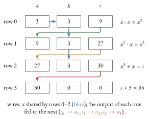
The table as printed does not yet encode the computation. Nothing forces the x
in row 0 to equal the x in rows 1 and 2 , nor the output
| a 0 = b 0 = b 1 = b 2 ⏟ all are x = 3, c 0 = a 1 ⏟ x 2 = 9, c 1 = a 2 ⏟ x 3 = 27, c 2 = a 3 ⏟ s = 30, |
where a j denotes the cell of column a in row j . Figure 2 draws them as wires. They turn a list of unrelated gates into a single dataflow; enforcing them is an argument in its own right, the permutation argument of §2.6.
Satisfiability of the grid.
The claim is now equivalent to a purely combinatorial assertion:
there exist values for the advice cells
2.2 From the grid to polynomials
The grid has finitely many rows, and the aim is a statement about all rows at once that the verifier can check at one point. A polynomial of degree less than n is determined by its values at n distinct points (Math Guide, §“Lagrange interpolation”), and the rest of the section relies on this.
An index set for the rows.
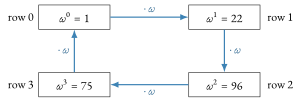
The table has
| H = { ω 0, ω 1, ω 2, ω 3 } = { 1, 22, 96, 75 } = { 1, 22, − 1, − 22 }, |
and row i lives at the point ω i (Figure 3).
Roots of unity are chosen
because they form a cyclic group: the row after ω i is
Columns become polynomials.
Each column of the table is four numbers, one per row. Interpolate: for
the advice column a there is a unique polynomial a (X) of degree
| a (ω 0) = 3, a (ω 1) = 9, a (ω 2) = 27, a (ω 3) = 30 |
(Math Guide, §“Lagrange interpolation”), and likewise b (X) ,
c (X) , the publicly known selector polynomials
| a (X) | = 90 + 61 X + 22 X 2 + 24 X 3, | q M (X) | = 49 + 19 X + 30 X 3, | ||
| b (X) | = 75 + 32 X + 25 X 2 + 65 X 3, | q L (X) | = 49 + 78 X + 67 X 3, | ||
| c (X) | = 65 + 16 X + 3 X 2 + 22 X 3, | q R (X) | = 73 + 24 X + 73 X 2 + 24 X 3, | ||
| PI (X) | = 64 + 50 X + 33 X 2 + 47 X 3, | q O (X) | = 72 + 54 X + 24 X 2 + 43 X 3, | ||
| q C (X) | = 74 + 76 X + 23 X 2 + 21 X 3, | ||||
and each returns its column at the rows: b takes the values
(3, 3, 3, 0) on H , q O the values (96, 96, 96, 0) , and
PI the values (0, 0, 0, 62) . Interpolation is thus a
bijection between columns of four values and polynomials of degree
The gate polynomial.
Assemble the left-hand side of the gate equation (1) with the polynomials in place of the per-row numbers.
Theorem 2.1 (The gate polynomial).
Let
| G (X) := q M (X) a (X) b (X) + q L (X) a (X) + q R (X) b (X) + q O (X) c (X) + q C (X) + PI (X) . | (2) |
Then
Proof.
The term q M a b multiplies three polynomials of degree at most 3 , and
every other term has degree at most 6 , so
For the honest trace,
| G (X) = 36 + 27 X + 54 X 2 + 50 X 3 + 77 X 4 + 24 X 5 + 43 X 6 + 47 X 7 + 81 X 8 + 46 X 9, |
of degree exactly 9 , and it vanishes at all four points of H by construction. “Every gate is satisfied” has become “ G vanishes on H ”; the copy constraints remain separate. Four separate checks are now one statement about one polynomial.
2.3 From vanishing to a single identity
The condition “ G vanishes on H ” is still a statement about four points. This subsection replaces it by a polynomial identity that refers to no individual row.
The vanishing polynomial.
The vanishing polynomial of H is the monic polynomial (leading coefficient 1 ) whose roots are exactly the points of H ,
| Z H (X) := ∏ i = 0 3 (X − ω i) = X 4 − 1, |
where the closed form
Theorem 2.2 (Gate satisfaction is a quotient).
Every gate of the trace holds if and only if there is a polynomial t (X)
with
Proof.
By Theorem 2.1, every gate holds if and only if
G vanishes on H . The factor theorem (Math Guide, §“Roots and
the factor theorem”) gives
| G vanishes on H ⇔ (X − ω i) ∣ G for each i ⇔ Z H (X) ∣ G (X), | (3) |
and divisibility is the existence of the quotient t . □
Satisfaction of the gate constraints is precisely the existence of t ; correct wiring still requires the copy constraints. For the honest trace the division comes out even: G has degree 9 , Z H has degree 4 , and
| t (X) = G (X) X 4 − 1 = 61 + 70 X + 43 X 2 + 47 X 3 + 81 X 4 + 46 X 5 |
is a polynomial of degree 5 with remainder zero, as it must be.
Example 2.3 (Why a cheat cannot produce t ).
Suppose the advice is wrong: some gate fails. Then G does not vanish on
all of H , so by (3) Z H does not divide G , and
no polynomial t satisfies
| G ∗ (X) = 54 + 10 X + 43 X 2 + 74 X 3 + 83 X 4 + 65 X 5 + 78 X 6 + 47 X 7 + 81 X 8 + 46 X 9 . |
Dividing G ∗ by Z H with remainder (Math Guide, §“Division
with remainder”) gives the quotient
| D (X) = 24 (1 + X + X 2 + X 3), | (4) |
of degree 3 . The identity
2.4 Why checking one random point is a proof
The prover wishes to convince the verifier that
Construction 2.4 (The random-point check).
-
1.
The prover commits to her polynomials
a, b, c and to the quotient t ; the selector and public-input polynomials the verifier already knows. -
2.
The verifier picks a point
z ∈ F uniformly at random and sends it. -
3.
The prover opens her commitments at z : she returns the field elements
a (z), b (z), c (z), t (z) together with short proofs that these are the true evaluations of the committed polynomials. -
4.
The verifier forms G (z) from the openings and the self-evaluated public polynomials via (2), computes
Z H (z) = z 4 − 1 , and checks the single field equation G (z) = ? t (z) Z H (z) . (5)
He accepts if and only if (5) holds.
The honest case (completeness).
If the prover is honest then
| Z H (20) = 20 4 − 1 = 46, t (20) = 67, G (20) = 75 = 67 ⋅ 46 = t (20) Z H (20), |
and the verifier accepts. He accepts every time, for every z .
The dishonest case (soundness).
Soundness rests on the fact that a nonzero polynomial of low degree has few roots.
Theorem 2.5 (Soundness of the random-point check).
Suppose the trace is invalid, so that the prover’s gate polynomial G ∗
does not vanish on all of H , and let t ∗ be any polynomial she
commits to as the quotient. Set
| Pr z [the verifier accepts] = Pr z [D (z) = 0] ≤ deg D | F | . |
Proof.
Were D the zero polynomial,
The bound deg D / | F | is negligible when | F | is exponential in the security parameter and deg D is polynomial in it. The verifier does not recompute the trace; he tests one polynomial identity at one random point.
Example 2.6 (The random-point check on the toy).
For the
| Pr [cheat accepted] = 3 97 . |
At the actual draw
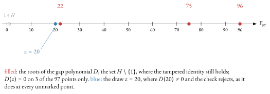
Scale.
The fraction 3 / 97 is large only because the field is a toy, and it concerns one particular quotient; the next paragraph bounds every cheat by 11 / 97 . What such a term means at the deployed field size is the scale caveat of §1.2.
Bounding the degree.
The argument needs deg D small relative to | F | , otherwise
“ deg D roots out of | F | ” is no constraint at all. The commitment
scheme enforces a degree bound on every committed polynomial
(Crypto Guide, §“Polynomial commitment schemes”), so the prover
cannot commit to a t ∗ of unbounded degree. The bound follows the
degree the commitment admits, not the honest degree. The wires are
committed at degree below
2.5 PLONKish arithmetisation
The toy has met every ingredient concretely: an evaluation domain H , a
generator ω , the vanishing polynomial Z H , columns interpolated
into polynomials of degree
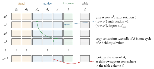
Definition 2.7 (PLONKish constraint system).
Fix a prime field F and an integer k with
-
1.
a finite set Col of columns, each of n cells, one per row, partitioned into fixed columns (preprocessed circuit data, known to both parties), advice columns (the prover’s witness) and instance columns (public input); a cell is an element of
H × Col , and the circuit assigns every cell of a fixed column its value; -
2.
a maximum constraint degree d max ;
-
3.
a finite set
R ⊂ Z of rotations containing 0 ; a column expression is a polynomial over F in the values v (ω r X) for v ∈ Col and r ∈ R , where the value of v at rotation r at row i is the cell of v in row i + r taken modulo n ; -
4.
a finite sequence of custom gates
g j = 0 , each g j a column expression of degree at most d max ; -
5.
a set
H act ⊆ H of active rows: all of H in the toy, and in the deployed system the first u < n rows ω 0, ..., ω u − 1 , the trailing rows being reserved for a boundary row and blinding (Remark 2.17 fixes u ); -
6.
a subset
E ⊆ H act × Col of equality-constrained cells together with a permutation σ of E (a bijection E → E ) whose cycles, the orbits { κ, σ (κ), σ 2 (κ), ... } of the cells κ ∈ E , are the classes of cells required to hold a common value; -
7.
a set of lookup arguments, each an input tuple (A 0, ..., A m − 1) of column expressions and a table tuple (S 0, ..., S m − 1) of columns.
An assignment gives every cell a value in F , the fixed cells
their circuit values; write v κ for the value of cell κ . It
is satisfying if every gate vanishes at every row of H (in the
deployed system the selectors are zero outside H act ),
The letter d is reserved, from §3 on, for the length of a committed vector; the constraint degree is therefore written d max throughout this volume.
Vanilla PLONK as the special case.
The original PLONK system of Gabizon, Williamson and Ciobotaru uses a single fixed five-selector universal gate,
| q M (X) a (X) b (X) + q L (X) a (X) + q R (X) b (X) + q O (X) c (X) + q C (X) + PI (X) ≡ 0 (mod Z H (X)), |
with three wire polynomials
Columns as committed polynomials.
With the Lagrange basis l j (X) of H , defined by
2.6 Enforcing the wiring: the permutation argument
The copy constraints of §2.1 remain to be enforced.
The gate identity of §§2.2–2.4
checks each row separately; it does not assert that
Equalities as a permutation.
Group the cells into the classes that must share a value, { a 0, b 0, b 1, b 2 } , { c 0, a 1 } , { c 1, a 2 } , { c 2, a 3 } , and let σ be the permutation of the twelve cells that cycles each class in the order written and fixes b 3 and c 3 :
| a 0 → b 0 → b 1 → b 2 → a 0, c 0 ↔ a 1, c 1 ↔ a 2, c 2 ↔ a 3 . |
Give every cell a distinct label: the cell in row j of the a -,
b -, c -column gets ω j , k 1 ω j , k 2 ω j
respectively, where
| H = { 1, 22, 96, 75 }, 2 H = { 2, 44, 95, 53 }, 3 H = { 3, 66, 94, 31 } . |
Write λ cell for a cell’s label and v cell
for its value. Asserting “cells in a class are equal” is then
equivalent to asserting that the multiset (a finite collection in
which an element may occur more than once; two multisets are equal when
every element occurs equally often in both) of pairs
{ (v cell, λ cell) } is unchanged when each
label is replaced by the label of the cell’s image under σ : a pair
(v, λ) moves to (v, λ σ) , and the moved pair was already
present exactly when the cell at λ σ carried the same value v .
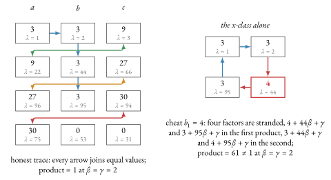
Figure 6 draws the cycles with their labels. Because
labels are distinct, comparing two multisets of pairs is a job for a
product: compress each pair to the linear form
| ∏ cells (v cell + β λ cell + γ) against ∏ cells (v cell + β λ σ (cell) + γ) . | (6) |
If the wiring is honest the two products run over the same multiset of
factors and agree identically in
The running product.
A product over all cells is not a local fact, so the prover commits to a
running product: a column Z perm with
A single wired pair.
Strip the product down to a single wired pair,
| (9 + β λ c 0 + γ) (9 + β λ a 1 + γ) = (9 + β λ a 1 + γ) (9 + β λ c 0 + γ), |
because the shared value 9 makes the two left-hand factors a mere
reordering of the two right-hand ones: the labels may permute under
σ precisely because the values agree. Now let the prover cheat the
copy,
Example 2.8 (The permutation check on the toy).
For the honest trace with
The general argument.
Halo 2 states the argument for any number of columns, and the statement needs one lemma on two-variable polynomials. The Schwartz–Zippel lemma of the Math Guide (§“The Schwartz–Zippel lemma”) is univariate; that section’s remark on the multivariate generalisation states the several-variable bound without proof, as a consequence of the univariate lemma applied once per variable, and Lemma 2.9 carries out that derivation for two variables.
Lemma 2.9 (Two variables).
Let
Proof.
Write
Construction 2.10 (Permutation argument over m columns).
Let
| l 0 (X) (1 − Z perm (X)) | ≡ 0, | (7) | ||
| Z perm (ω X) ∏ i = 0 m − 1 (v i (X) + β s i (X) + γ) − Z perm (X) ∏ i = 0 m − 1 (v i (X) + β δ i X + γ) | ≡ 0, |
which together assert
| ∏ i, j (v i (ω j) + β δ i ω j + γ) = ∏ i, j (v i (ω j) + β s i (ω j) + γ) . | (8) |
The verifier opens Z perm at the random point z and at ω z , and checks the boundary and the cross-multiplied update.
The first identity fixes
Theorem 2.11 (Soundness of the permutation argument).
The assignment satisfies every equality constraint (cells related by
σ carry equal values) if and only if the two sides
of (8) are equal as polynomials in β and
γ . Consequently the honest prover always satisfies
(8), and if some constraint is violated the two
sides agree at uniformly random
Proof.
Index cells by κ , write v κ and λ κ for value and label, and set
| P (β, γ) := ∏ κ (γ + v κ + β λ κ) − ∏ κ (γ + v κ + β λ σ (κ)) ∈ F [β] [γ] . |
Each side is a product of monic linear polynomials in γ over the
ring F [β] , with roots
If every constraint holds then
If some constraint fails, pick κ 0 with
The honest prover’s ratio is 1 whenever the denominator is nonzero. The deployed boundary rule of Remark 2.17 admits the final value 0 , and the error bound changes accordingly.
Corollary 2.12 (Permutation argument under the deployed boundary rule).
Let the columns be fixed before
Proof.
Suppose some running products satisfy the identities and no numerator
factor
Cost.
Excluding the final commitment check, the verifier’s work for the
argument is
The deployed chunking.
The update identity in (7) has degree
2.7 Proving a value sits in a table: lookups
Some constraints admit no low-degree gate on the constrained cells alone.
“This cell is a ten-bit number” or “this chunk indexes an entry of the
Sinsemilla generator table” (Sinsemilla is the hash of the Crypto
Guide, §“Sinsemilla: an algebraic hash-based commitment”) has no
low-degree formula in the cell itself: written as one polynomial gate,
“
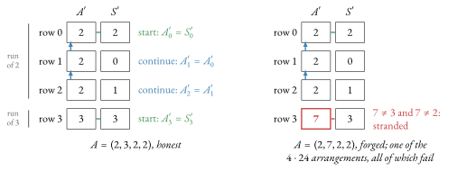
Membership of every entry of a column A in a table column S is, like
a copy constraint, a statement about multisets, but it is not a
permutation: A may repeat one table entry and omit others. The prover
therefore commits to A ′ , a rearrangement of A in which equal values
occupy contiguous runs, and to S ′ , a rearrangement of S in
which the first row of each run of A ′ holds the matching table value.
Two row-local conditions then give membership: each row of A ′
either begins a run,
Example 2.13 (A two-bit range check on the toy grid).
Constrain cells to two-bit values with the table
The Action circuit uses lookups of both kinds: it range-constrains each
ten-bit word of a decomposition by a lookup into the table
2.8 The lookup argument
Construction 2.14 (Lookup argument).
The objective is that every entry of the column A (X) on the active rows
appears as some entry of the column S (X) (the halo2 book’s
Lookup argument chapter). The prover supplies
polynomials A ′ (X) and S ′ (X) where (i) A ′ is a permutation of A
with like values grouped into contiguous runs, and (ii) S ′ is a
permutation of S in which the first row of each run of like values in
A ′ holds the matching value. The prover commits to A ′ and S ′ ;
after receiving challenges
| l 0 (X) (1 − Z lookup (X)) | ≡ 0, | (9) | ||
| Z lookup (ω X) (A ′ (X) + β) (S ′ (X) + γ) − Z lookup (X) (A (X) + β) (S (X) + γ) | ≡ 0, | |||
| l 0 (X) (A ′ (X) − S ′ (X)) | ≡ 0, | |||
| (A ′ (X) − S ′ (X)) (A ′ (X) − A ′ (ω − 1 X)) | ≡ 0, |
the second and fourth additionally masked by the active-row factor of Remark 2.17.
Theorem 2.15 (Soundness of the lookup argument).
Let the columns
Proof.
Let the active rows be
| ∏ i < u (A i ′ + β) (S i ′ + γ) = ∏ i < u (A i + β) (S i + γ) . |
Set
So, with that probability excepted, A ′ is a rearrangement of A and S ′ of
S on the active rows. The third identity fixes row 0 :
Multi-column tables.
A lookup of m input expressions
| A c (X) := ∑ j = 0 m − 1 θ m − 1 − j A j (X), S c (X) := ∑ j = 0 m − 1 θ m − 1 − j S j (X), | (10) |
and Construction 2.14 runs on A c and S c .
Proposition 2.16 (Compression of a multi-column lookup).
Let θ be drawn uniformly after all input and table columns are
fixed. If the input tuple at some active row equals the table tuple at no
active row, then the compressed input A c at that row equals
S c at some active row with probability at most
Proof.
For each active table row the difference of the compressed values is a
polynomial in θ of degree at most
Variable tables, where S is itself an advice column, and range checks, where S enumerates the allowed range, are special cases of the same argument.
Remark 2.17 (Active rows and blinding).
The lookup identities, like the permutation identities of
§2.6, hold on the active rows only. The deployed
system withholds the trailing rows of every column from them: a boundary
row and, after it, n blind blinding rows, which in every
witness column (advice, and the permuted and running-product columns of
the arguments) hold uniform random values, for the reason “Zero
knowledge: hiding the witness in Halo 2” in §4 gives;
fixed and instance columns carry no random values. Let
2.9 Why the prover cannot wriggle: binding commitments
The random-point argument of §2.4 rests on a hypothesis:
Theorem 2.5 assumed the prover’s polynomials were fixed
before she saw z . If she could choose
What a commitment must do.
A commitment to a polynomial f is a short string
-
•
Binding. Having published C , the prover cannot later open it as two different polynomials; C pins down f . Committing first, then receiving z , then opening, leaves her answering for the one polynomial she fixed in advance, the situation Theorem 2.5 assumed.
-
•
Hiding. The string C reveals nothing about f . This is what will let the proof be zero-knowledge, under “Zero knowledge: hiding the witness in Halo 2” in §4.
A polynomial commitment adds an evaluation proof: given C and a
point z , the prover can prove “
How Halo 2 commits.
Encode f of degree
| C = ⟨ f, G ⟩ + [r] H = ∑ i [f i] G i + [r] H, |
the Pedersen vector commitment of the coefficient vector with blinder
| f (z) = ∑ i f i z i = ⟨ f, (1, z, z 2, ..., z n − 1) ⟩, |
and the inner-product argument does this in a logarithmic number of rounds, each halving the vectors, until the claim is trivial: the evaluation proof is O (log n) group elements, and it needs no trusted setup, because the generators come from a public hash rather than from anyone’s secret (Crypto Guide, §“Polynomial commitment schemes”, the inner-product alternative). Halo 2 uses exactly this one polynomial commitment scheme and no other: the inner-product argument (the halo2 book, which the protocol specification names as the definition of the system, § 5.4.10.3, “Halo 2”; its Inner product argument chapter), on the Vesta curve, where the protocol specification places the Action statement’s proofs (protocol specification, § 5.4.9.6, “Pallas and Vesta”). The parameters, the generators and the deployed byte layout are given at the end of §3.
Opening a vector commitment.
For the argument of this section the commitment must bind, so that the
prover answers for polynomials fixed before z is drawn. A vector
commitment alone does not provide step 3 of the random-point check. The
only opening the Pedersen construction offers is the whole vector
together with its blinder,