9 Roots of unity and evaluation domains
This section constructs the evaluation domains on which polynomial proof
systems of the kind underlying Halo 2 and Zcash Orchard encode computations,
and the fast Fourier transform on them. Such a proof system records an
n -step computation as a table over a finite field, one column per
register and one row per step, and convinces a verifier that every row
follows from its predecessor without the verifier replaying the
computation: by Lagrange interpolation (5.30)
each column is the value table on n fixed points of a polynomial of
degree less than n , so conditions on the table become polynomial
identities, checkable at a single random point by the Schwartz–Zippel
lemma (5.45). The powers of a
primitive n -th root of unity form a point set on which conditions on
every row, shifts to the next row and the polynomials attached to the set are
cheap to evaluate, and on which conversion between values and
coefficients, and polynomial multiplication, cost far fewer than the
n 2 field operations of the schoolbook methods. Such a root exists in
F q exactly when
Throughout, F denotes a field. When F is to be finite, the
notation F q denotes the field with q elements (so q is a
prime power, 6.10); when we intend a prime
field specifically we write F p . The multiplicative group of nonzero
elements is
9.1 Roots of unity
Definition 9.1 (Root of unity).
Let F be a field and
| μ n (F) = { ω ∈ F : ω n = 1 } |
for the set of all n -th roots of unity in F .
Since
Proposition 9.2.
The set μ n (F) is a finite subgroup of F × of order at most n .
Proof.
The identity 1 satisfies
The bound
Definition 9.3 (Primitive root of unity).
An element
The order ord (ω) is the least positive integer d with
Remark 9.4 (Primitive roots as roots of unity).
The group-theoretic term “generator of F q × ” and the
polynomial term “primitive
Lemma 9.5 (Order divides exponent).
Let
Proof.
The first claim is 3.12(1), read in the
abelian group F × : if
Proposition 9.6.
If
| μ n (F) = ⟨ ω ⟩ = { 1, ω, ω 2, ..., ω n − 1 } |
is a cyclic group of order exactly n , and these n powers are pairwise distinct.
Proof.
The powers
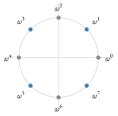
Over the complex numbers a primitive n -th root of unity always
exists, namely
9.2 Existence over finite fields: the condition
n ∣ q − 1
The multiplicative group F q × of a finite field is cyclic of
order
Theorem 9.7 (Existence and count of primitive n -th roots of unity).
Let F q be a finite field and
-
1.
The field F q contains a primitive n -th root of unity if and only if
n ∣ q − 1 . -
2.
When
n ∣ q − 1 , the group μ n (F q) is cyclic of order exactly n , and the number of primitive n -th roots of unity in F q is φ (n) , where φ is Euler’s totient function (2.26).
Proof.
Let g be a generator of F q × , which is cyclic of order
( ⇒ ) Suppose ω is a primitive
n -th root of unity in F q . Then
( ⇐ ) Suppose
| ord (ω) = ord (g m) = ord (g) gcd (m, ord (g)) = q − 1 gcd (m, q − 1) = q − 1 m = n, |
using the order-of-a-power formula
(Corollary 3.23) together with
Count. In the cyclic group
(On the coprimality hypothesis. The condition
Remark 9.8.
The proof shows that for a finite field the statement reduces to
F q has a primitive n -th root of unity
Example 9.9.
Take
Remark 9.10 (Two-adicity and FFT-friendly primes).
For the fast algorithms below, n should be a power of two, or at
least smooth—a product of small primes, ideally with many
factors of two. By 9.7, a primitive
2 k -th root of unity exists exactly when
9.3 The evaluation domain H and its vanishing polynomial
Definition 9.11 (Evaluation domain).
Let F be a field containing a primitive n -th root of unity ω . The evaluation domain of order n is the multiplicative subgroup
| H = ⟨ ω ⟩ = { 1, ω, ω 2, ..., ω n − 1 } = μ n (F) ⊆ F ×, |
a cyclic group of order n by 9.6. We
index its elements as
Definition 9.12 (Vanishing polynomial).
The vanishing polynomial (or zerofier) of H is
| Z H (X) = ∏ h ∈ H (X − h) ∈ F [X] . |
On a generic n -point set the vanishing polynomial (5.33) is a product of n linear factors with no simpler form; on the group H it reduces to a binomial.
Theorem 9.13 (Closed form and factorisation of the vanishing polynomial).
With
| Z H (X) = X n − 1 = ∏ i = 0 n − 1 (X − ω i) . |
Moreover Z H is separable: it has n distinct roots and
Proof.
Every
For separability, the formal derivative is
The proof shows that
Proposition 9.14 (Cosets and shifts).
Let
| Z γ H (X) = ∏ h ∈ H (X − γ h) = X n − γ n . |
In particular, distinct cosets of H in F × have vanishing
polynomials
Proof.
Substitute
| ∏ h ∈ H (X − γ h) = γ n ∏ h ∈ H (Y − h) = γ n (Y n − 1) = γ n ((X / γ) n − 1) = X n − γ n, |
using 9.13 for the middle equality. The
constant is
| γ 1 H = γ 2 H ⇔ γ 1 / γ 2 ∈ H ⇔ (γ 1 / γ 2) n = 1 ⇔ γ 1 n = γ 2 n, |
so distinct cosets give distinct constants c . □
Lemma 9.15 (Finite geometric series).
Let F be a field,
| ∑ i = 0 n − 1 ζ i = ζ n − 1 ζ − 1 . |
Proof.
Write
| ζ S = ζ + ζ 2 + ⋯ + ζ n − 1 + ζ n . |
In the difference
| (ζ − 1) S = ζ S − S = ζ n − 1 . |
Since
Proposition 9.16 (Sum of roots of unity).
If
| ∑ i = 0 n − 1 ω k i = { n if n ∣ k, 0 if n ∤ k . |
Proof.
If
| ∑ i = 0 n − 1 ζ i = ζ n − 1 ζ − 1 = (ω n) k − 1 ζ − 1 = 1 − 1 ζ − 1 = 0, |
the denominator being nonzero because
Remark 9.17 (Vanishing by rotation invariance).
For
Remark 9.18 (Why “orthogonality”).
Call two vectors in F n orthogonal when their standard
inner product (8.21) vanishes. For each frequency
k let
9.4 The Lagrange basis on H
Since H has exactly n points, values on H determine polynomials of degree less than n (5.20); the basis adapted to values on H is the Lagrange basis of §5.7.
Definition 9.20.
For each
| L i (X) = ∏ j = 0 j ≠ i n − 1 X − ω j ω i − ω j ∈ F [X] < n, |
the basis polynomial l i of 5.30 for
the nodes
Proposition 9.21 (Interpolation property).
The polynomials
| L i (ω j) = δ i j = { 1 i = j, 0 i ≠ j, |
they form a basis of F [X] < n , and they give the unique
interpolant: for any data
| f (X) = ∑ i = 0 n − 1 v i L i (X) |
is the unique element of F [X] < n with
Proof.
Each L i is well defined and of degree
The root-count step recurs and is called the root-count device:
two polynomials of degree
On a generic point set the Lagrange polynomials admit no closed form simpler than the defining product; on the group H they are expressed through the vanishing polynomial.
Theorem 9.22 (Closed form of the Lagrange basis on H ).
For
| L i (X) = ω i n ⋅ X n − 1 X − ω i = ω i (X n − 1) n (X − ω i) . |
In particular, dividing out one linear factor and scaling yields all
n Lagrange polynomials from the single polynomial
Proof.
Fix i . From 9.13,
| Z H (X) X − ω i = ∏ j = 0 j ≠ i n − 1 (X − ω j), |
which is exactly the numerator of L i in
9.20. It remains to evaluate the
denominator
| Z H ′ (ω i) = g (ω i) = ∏ j = 0 j ≠ i n − 1 (ω i − ω j) |
—the derivative at a simple root equals the product of the
differences to the other roots, the computation already made for simple
roots in the proof of 5.40. Concretely
| Z H ′ (ω i) = n (ω i) n − 1 = n ω i n ω − i = n ⋅ 1 ⋅ ω − i = n ω i, |
using
| L i (X) = Z H (X) / (X − ω i) Z H ′ (ω i) = (X n − 1) / (X − ω i) n / ω i = ω i (X n − 1) n (X − ω i), |
as claimed. □
Remark 9.23 (Barycentric form).
The closed form gives the barycentric interpolation formula on
H a compact form. Writing
| f (X) = X n − 1 n ∑ i = 0 n − 1 ω i v i X − ω i . |
Evaluating f at a point
Proposition 9.24 (Lagrange polynomials sum to one).
The Lagrange basis polynomials for H satisfy
Proof.
Example 9.25 (The all-ones value vector).
The constant polynomial 1 interpolates the data
9.5 Evaluation and interpolation as mutually inverse linear maps
An element of F [X] < n is described by its n coefficients or by its n values on H ; passage between these two coordinate systems is a linear isomorphism, the specialisation to H of the evaluation isomorphism for general nodes in 5.32.
Definition 9.26 (Evaluation map).
The evaluation map on H is the F -linear map (8.18)
| ev H : F [X] < n ⟶ F n, ev H (f) = (f (ω 0), f (ω 1), ..., f (ω n − 1)) . |
Linearity is immediate from
Theorem 9.27 (Evaluation and interpolation are mutually inverse).
The evaluation map ev H is a vector-space isomorphism. Its inverse is the interpolation map
| int H : F n ⟶ F [X] < n, int H (v 0, ..., v n − 1) = ∑ i = 0 n − 1 v i L i (X) . |
That is,
Proof.
Both maps are linear and act between spaces of the same finite
dimension n , so verifying one composition would suffice (a
one-sided inverse makes ev H injective, hence surjective by
rank–nullity, 8.19); we verify both. For
In coordinates, ev H is given by a matrix, which identifies
evaluation on H with the Fourier transform. Matrix notation is fixed
as follows: an
Definition 9.28 (Vandermonde / DFT matrix).
Let
| V = (ω i k) 0 ≤ i, k ≤ n − 1 = (1 1 1 ⋯ 1 1 ω ω 2 ⋯ ω n − 1 1 ω 2 ω 4 ⋯ ω 2 (n − 1) ⋮ ⋮ 1 ω n − 1 ω 2 (n − 1) ⋯ ω (n − 1) 2) |
—rows indexed by the evaluation point ω i , columns by the
power k —represents ev H , so that
Theorem 9.29 (Invertibility and the inverse transform).
The matrix V of 9.28 is invertible, with
| (V − 1) k, i = 1 n ω − i k . |
Equivalently,
| c k = 1 n ∑ i = 0 n − 1 f (ω i) ω − i k, f (ω i) = ∑ k = 0 n − 1 c k ω i k . |
Proof.
First,
| ∑ i = 0 n − 1 ω − i k ω i k ′ = ∑ i = 0 n − 1 ω i (k ′ − k) . |
By 9.16 this sum is n if
9.6 The number-theoretic transform and convolution
The map ev H , read as the matrix V , is the discrete Fourier transform over a finite field rather than over C ; since it involves no analytic structure (no complex exponentials, no convergence), it is called the number-theoretic transform.
Definition 9.31 (Number-theoretic transform).
Let ω be a primitive n -th root of unity in F . The
number-theoretic transform (NTT) sends the coefficient vector
of a polynomial to its value vector on H : it is the evaluation map
ev H written in coordinates. Explicitly, the NTT of
| a ^ j = ∑ k = 0 n − 1 a k ω j k, j = 0, ..., n − 1, |
each entry being the value at ω j of the polynomial with coefficients a . The inverse number-theoretic transform is interpolation—the recovery of the coefficients from the values—and by 9.29 it too is a single explicit sum:
| a k = 1 n ∑ j = 0 n − 1 a ^ j ω − j k . |
The NTT has the convolution property of the classical DFT, the basis of
fast polynomial multiplication. The coefficients of a product are a
convolution: with
| (a ∗ b) k = ∑ 0 ≤ i, j ≤ n − 1 i + j ≡ k (mod n) a i b j, k = 0, ..., n − 1 . |
Theorem 9.32 (Convolution theorem).
For
| c (h) = f (h) g (h), |
i.e. pointwise multiplication of value vectors corresponds to
polynomial multiplication. Equivalently, writing
| a ∗ b ^ j = a ^ j b ^ j (j = 0, ..., n − 1), |
so the NTT turns convolution into entrywise multiplication.
Proof.
The first identity is the statement that evaluation at h is a ring
homomorphism
The convolution statement is proved in three steps: (i) multiplication in
Next consider the map
Remark 9.33 (Computational significance).
9.32 reduces multiplying two
degree-
Example 9.34 (The convolution theorem in F 17 ).
In F 17 , the element
9.7 The fast Fourier transform
Computing
Theorem 9.35 (Cooley–Tukey radix-2 step).
Suppose
| f even (Y) = ∑ k = 0 m − 1 a 2 k Y k, f odd (Y) = ∑ k = 0 m − 1 a 2 k + 1 Y k, |
so that
| f (ω j) | = f even (η j) + ω j f odd (η j), | (7) | ||
| f (ω j + m) | = f even (η j) − ω j f odd (η j) . | (8) |
Thus the length- n NTT of a reduces to two length- m NTTs (of the even and odd coefficient subsequences, over the domain ⟨ η ⟩ ) plus O (n) extra operations.
Proof.
The identity
It remains to evaluate. For (7), put
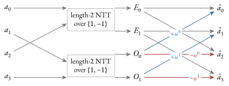
Remark 9.36 (The butterfly).
Equations
(7)–(8)
constitute the butterfly: from the two subtransform outputs
Theorem 9.37 ( O (n log n) cost of the FFT).
Let
| T (n) = 2 T (n / 2) + c n (n > 1), T (1) = O (1), |
for a constant c , and therefore
Proof.
The recursion is exactly 9.35: a length- n
transform calls two length- n / 2 transforms (on the even and odd
coefficient subsequences) and combines them with n / 2 butterflies of
O (1) operations each, for the c n overhead. Unrolling, with
| T (2 t) = 2 T (2 t − 1) + c 2 t . |
Divide by 2 t and set
Remark 9.38 (Mixed radix and smoothness).
Fast transforms apply when n is smooth and the field contains a
primitive n -th root of unity, that is,
Example 9.39 (A length- 4 transform).
Take
| E = (a 0 + a 2, a 0 − a 2), O = (a 1 + a 3, a 1 − a 3), |
and the butterflies give
| a ^ 0 = E 0 + ω 0 O 0, a ^ 2 = E 0 − ω 0 O 0, a ^ 1 = E 1 + ω 1 O 1, a ^ 3 = E 1 − ω 1 O 1 . |
(Outputs j and
9.8 The role of smooth multiplicative domains in polynomial proof systems
This subsection states how the preceding results are used in Halo 2,
the proof system of Orchard, which encodes a computation as polynomial
identities on the evaluation domain
Remark 9.40 (The roles played by H , Z H , the Lagrange basis, and the FFT).
-
•
Witnesses as evaluations on H . A prover lays out the trace of a computation as the values of one or more polynomials on the n points of H . By 9.27 this is the same data as a polynomial of degree
< n ; the prover may move freely between the value (Lagrange) representation, suited to stating constraints row by row, and the coefficient representation, suited to committing and to low-degree testing. The change of representation is the (inverse) NTT. -
•
Constraints as divisibility by Z H . “Constraint polynomial C holds on every row” means C vanishes on all of H , which by 9.13 means exactly that
Z H = X n − 1 divides C . The prover demonstrates this by exhibiting a quotient t with C (X) = t (X) (X n − 1) . The closed form Z H (X) = X n − 1 , evaluated by one exponentiation, makes this check cheap at a random point. 9.14 extends the same technique to cosets γ H , used to separate quotient and remainder domains. -
•
Lagrange selectors. The Lagrange polynomials L i of 9.20 are selectors: L i is 1 on row i and 0 elsewhere (9.21), so boundary and instance constraints (e.g. “the first row equals the public input”) become
L 0 ⋅ (...) . The closed form and the barycentric formula (9.22, 9.23) let the verifier evaluate these at a random challenge in O (n) or even O (log n) field operations rather than reconstructing polynomials. -
•
Group structure for permutations and shifts. Because H is a cyclic group (9.11), multiplication by ω is the cyclic “next-row” shift
ω i ↦ ω i + 1 . Constraints relating a row to its neighbour become f (ω X) versus f (X) ; permutation arguments, on which Halo 2’s copy constraints are built, rest on the action of the group on itself and on its cosets. An arbitrary set of n points has none of this structure. -
•
Smoothness for speed. Provers manipulate polynomials of size n (often after enlarging the domain by a small constant factor for low-degree testing). Transforms between representations, multiplications and coset evaluations are computed by NTTs, which by 9.37 cost O (n log n) instead of O (n 2) (at the sizes used in practice, the difference between feasible and infeasible computation), provided n is smooth and F q contains a primitive n -th root of unity. By 9.7 that requires
n ∣ q − 1 ; by 9.10 this is why high-two-adicity primes are chosen for the scalar fields of the Pallas and Vesta curves (10).